Analyze data collected through an interactive quiz, focused on couples planning their wedding. The main purpose is to segment these leads to better understand their profiles, needs, and stage in planning.
The main objective was to use unsupervised learning techniques (clustering) to identify distinct groups of couples based on their responses, allowing for the creation of more effective and personalized marketing strategies.
Project Structure
The development of this project followed a structured and iterative methodology, covering everything from data collection and preparation to the evaluation and interpretation of results.
Data Collection and Preparation
The initial phase involved the consolidation and cleaning of data. Leads were collected from three distinct sources, requiring a unification and standardization process to ensure dataset quality.
Data Loading and Concatenation
Data Source: Collection of online quiz responses, distributed across 03 CSV files.
Loading and Unification: Reading different files and consolidating them into a single dataset.
The columns created_at options: opcoes_UAa9JQ, code,button: oQcJxV, button: 0FvZw6, button: enviar and tracking do not contain relevant information for the analysis, so we can remove them from df01 and df02. The columns field: 11ABFZ, field: 3hxWeL, field: 5fSLVc contain data about the lead, but have too little data to work with, so we will also remove them from the dataframes..
We noticed that some answers have the letter A/B/C/D before the answer and other answers do not. We need to map both scenarios.
Mapping responses (with and without letter):
Show Code
# Dictionary to map responses with lettermapeamento_com_letra = {'(A) Ainda estamos completamente perdidos sobre tudo': 'A','(B) Temos algumas referências, mas nada decidido': 'B','(C) Já temos o estilo em mente, mas falta planejar': 'C','(D) Sabemos exatamente o que queremos e já começamos a organizar': 'D','(A) Vivemos no limite e temos dívidas': 'A','(B) Conseguimos nos manter, mas não sobra': 'B','(C) Temos folga, mas ainda não vivemos como gostaríamos': 'C','(D) Estamos bem financeiramente, mas queremos crescer mais': 'D','(A) Está completamente envolvido(a), sonha junto comigo': 'A','(B) Está envolvido(a), mas prefere que eu lidere': 'B','(C) Me apoia, mas não se envolve muito com o planejamento': 'C','(D) Prefere que eu resolva tudo sozinho(a)': 'D','(A) Não começamos ainda': 'A','(B) Temos anotações e ideias soltas': 'B','(C) Criamos um planejamento inicial, mas ainda sem orçamento': 'C','(D) Temos planilhas, metas e até cronograma definido': 'D','(A) Não conseguiríamos bancar nada ainda': 'A','(B) Conseguiríamos fazer algo simples': 'B','(C) Teríamos que parcelar bastante ou contar com ajuda': 'C','(D) Poderíamos arcar com boa parte, mas queremos mais liberdade': 'D','(A) Ainda não pensamos nisso': 'A','(B) Algo íntimo e simples, só com pessoas próximas': 'B','(C) Uma cerimônia encantadora, com tudo bem feito': 'C','(D) Um evento inesquecível, com tudo que temos direito': 'D','(A) Nem pensamos nisso ainda': 'A','(B) Pensamos, mas parece fora da nossa realidade': 'B','(C) Temos destinos em mente, mas sem orçamento ainda': 'C','(D) Já sabemos onde queremos ir e estamos nos planejando': 'D','(A) Desejamos, mas nos falta tempo e direção': 'A','(B) Queremos muito, mas temos medo de não dar conta': 'B','(C) Estamos dispostos, só falta um plano eficaz': 'C','(D) Estamos prontos, queremos agir e realizar de verdade': 'D'}# Dictionary to map responses without lettermapeamento_sem_letra = {'Ainda estamos completamente perdidos sobre tudo': 'A','Temos algumas referências, mas nada decidido': 'B','Já temos o estilo em mente, mas falta planejar': 'C','Sabemos exatamente o que queremos e já começamos a organizar': 'D','Vivemos no limite e temos dívidas': 'A','Conseguimos nos manter, mas não sobra': 'B','Temos folga, mas ainda não vivemos como gostaríamos': 'C','Estamos bem financeiramente, mas queremos crescer mais': 'D','Está completamente envolvido(a), sonha junto comigo': 'A','Está envolvido(a), mas prefere que eu lidere': 'B','Me apoia, mas não se envolve muito com o planejamento': 'C','Prefere que eu resolva tudo sozinho(a)': 'D','Não começamos ainda': 'A','Temos anotações e ideias soltas': 'B','Criamos um planejamento inicial, mas ainda sem orçamento': 'C','Temos planilhas, metas e até cronograma definido': 'D','Não conseguiríamos bancar nada ainda': 'A','Conseguiríamos fazer algo simples': 'B','Teríamos que parcelar bastante ou contar com ajuda': 'C','Poderíamos arcar com boa parte, mas queremos mais liberdade': 'D','Ainda não pensamos nisso': 'A','Algo íntimo e simples, só com pessoas próximas': 'B','Uma cerimônia encantadora, com tudo bem feito': 'C','Um evento inesquecível, com tudo que temos direito': 'D','Nem pensamos nisso ainda': 'A','Pensamos, mas parece fora da nossa realidade': 'B','Temos destinos em mente, mas sem orçamento ainda': 'C','Já sabemos onde queremos ir e estamos nos planejando': 'D','Desejamos, mas nos falta tempo e direção': 'A','Queremos muito, mas temos medo de não dar conta': 'B','Estamos dispostos, só falta um plano eficaz': 'C','Estamos prontos, queremos agir e realizar de verdade': 'D'}# Function to map responsesdef mapear_resposta(resposta, mapeamento_letra, mapeamento_sem):ifisinstance(resposta, str): resposta = resposta.strip() resposta_mapeada = mapeamento_letra.get(resposta)if resposta_mapeada:return resposta_mapeada resposta_mapeada = mapeamento_sem.get(resposta)if resposta_mapeada:return resposta_mapeada# Applies the function to all question columnscolunas_perguntas = ['pergunta_1', 'pergunta_2', 'pergunta_3', 'pergunta_4', 'pergunta_5', 'pergunta_6', 'pergunta_7', 'pergunta_8']df_gf[colunas_perguntas] = df_gf[colunas_perguntas].applymap(lambda resposta: mapear_resposta(resposta, mapeamento_com_letra, mapeamento_sem_letra))
Since we have a lot of NaN values, we decided to remove all rows that have all questions unanswered and then replace the rows that have NaN but not in all questions with the mode of each question.
Removing rows with null values:
Show Code
# Contar diretamente as linhas onde todas as colunas são NaNnum_linhas_todas_nan = df_gf.isna().all(axis=1).sum()# Remover linhas onde todas as colunas são NaNdf_gf= df_gf.dropna(how='all')# Verificando valores nulos novamenteprint(df_gf.isnull().sum())
Now let’s analyze the data to find the volume of missing values per question and how the answers are distributed for each question.
Calculating the percentage of missing values in each column:
Show Code
# Calculando o percentual de valores ausentes em cada colunapercentual_na_perguntas = df_gf.isna().mean() *100# Exibindo o percentual de valores ausentesprint(percentual_na_perguntas)
Let’s create a data dictionary in case it’s necessary to consult the questions and alternatives during the analysis.
Creating a dictionary with all questions and alternatives:
Show Code
perguntas_dict = {"pergunta_1": {"texto": "Nível de clareza sobre o casamento dos sonhos: Como vocês descreveriam o nível de clareza que têm sobre o casamento que desejam?","alternativas": {"A": "Ainda estamos completamente perdidos sobre tudo","B": "Temos algumas referências, mas nada decidido","C": "Já temos o estilo em mente, mas falta planejar","D": "Sabemos exatamente o que queremos e já começamos a organizar" } },"pergunta_2": {"texto": "Situação financeira atual: Como você descreveria a situação financeira atual de vocês dois?","alternativas": {"A": "Vivemos no limite e temos dívidas","B": "Conseguimos nos manter, mas não sobra","C": "Temos folga, mas ainda não vivemos como gostaríamos","D": "Estamos bem financeiramente, mas queremos crescer mais" } },"pergunta_3": {"texto": "Apoio mútuo e envolvimento no sonho de casamento: Como está o envolvimento do seu parceiro(a) na realização do casamento dos sonhos?","alternativas": {"A": "Está completamente envolvido(a), sonha junto comigo","B": "Está envolvido(a), mas prefere que eu lidere","C": "Me apoia, mas não se envolve muito com o planejamento","D": "Prefere que eu resolva tudo sozinho(a)" } },"pergunta_4": {"texto": "Nível de organização do planejamento: Como vocês estão se organizando para planejar o casamento?","alternativas": {"A": "Não começamos ainda","B": "Temos anotações e ideias soltas","C": "Criamos um planejamento inicial, mas ainda sem orçamento","D": "Temos planilhas, metas e até cronograma definido" } },"pergunta_5": {"texto": "Possibilidade de investimento atual no casamento: Se fossem realizar o casamento ideal hoje, como pagariam?","alternativas": {"A": "Não conseguiríamos bancar nada ainda","B": "Conseguiríamos fazer algo simples","C": "Teríamos que parcelar bastante ou contar com ajuda","D": "Poderíamos arcar com boa parte, mas queremos mais liberdade" } },"pergunta_6": {"texto": "Estilo de casamento desejado: Qual o estilo de casamento dos seus sonhos?","alternativas": {"A": "Ainda não pensamos nisso","B": "Algo íntimo e simples, só com pessoas próximas","C": "Uma cerimônia encantadora, com tudo bem feito","D": "Um evento inesquecível, com tudo que temos direito" } },"pergunta_7": {"texto": "Planejamento da lua de mel: Vocês já pensaram na lua de mel?","alternativas": {"A": "Nem pensamos nisso ainda","B": "Pensamos, mas parece fora da nossa realidade","C": "Temos destinos em mente, mas sem orçamento ainda","D": "Já sabemos onde queremos ir e estamos nos planejando" } },"pergunta_8": {"texto": "Comprometimento em tornar esse sonho realidade: O quanto vocês estão comprometidos em transformar esse sonho em realidade?","alternativas": {"A": "Desejamos, mas nos falta tempo e direção","B": "Queremos muito, mas temos medo de não dar conta","C": "Estamos dispostos, só falta um plano eficaz","D": "Estamos prontos, queremos agir e realizar de verdade" } }}
3. Model Building and Validation
The KMeans algorithm uses the Euclidean distance between points to form clusters. Euclidean distance is a measure of how far apart two points are in Euclidean space. Correlation can have a significant impact on clustering models like KMeans, as KMeans uses Euclidean distance between points to form clusters. Highly correlated variables can disproportionately influence the distances between points, leading to possible distortions in the formed clusters.
We need to consider multicollinearity (if two variables are highly correlated), the scale of variables (since KMeans is sensitive to scale), and dimensionality reduction (to speed up the grouping process when there are a large number of variables).
Therefore, before applying KMeans, let’s first analyze the correlation of categorical data. We will use Cramér’s V, which is a measure of association between two categorical variables, measuring how associated two nominal variables are.
Calculating Cramer’s V Matrix and performing the analysis:
Show Code
# Função para calcular Cramer's Vdef cramers_v(x, y): confusion_matrix = pd.crosstab(x, y) chi2 = chi2_contingency(confusion_matrix, correction=False)[0] n = confusion_matrix.sum().sum() phi2 = chi2 / n r, k = confusion_matrix.shape phi2corr =max(0, phi2 - ((k-1)*(r-1)) / (n-1)) rcorr = r - ((r-1)**2) / (n-1) kcorr = k - ((k-1)**2) / (n-1)return np.sqrt(phi2corr /min((kcorr-1), (rcorr-1)))# Criando matriz df = df_gfcategorical_columns = df.columns# Criar uma matriz vaziacramers_results = pd.DataFrame(np.zeros((len(categorical_columns), len(categorical_columns))), index=categorical_columns, columns=categorical_columns)# Preencher a matrizfor col1 in categorical_columns:for col2 in categorical_columns: cramers_results.loc[col1, col2] = cramers_v(df[col1], df[col2])# Imprimindo a mtrizcramers_results
pergunta_1
pergunta_2
pergunta_3
pergunta_4
pergunta_5
pergunta_6
pergunta_7
pergunta_8
pergunta_1
1.000000
0.154443
0.000000
0.353861
0.193979
0.174872
0.150004
0.261624
pergunta_2
0.154443
1.000000
0.080247
0.217220
0.319514
0.159740
0.196799
0.175146
pergunta_3
0.000000
0.080247
1.000000
0.104207
0.099763
0.079644
0.102016
0.105724
pergunta_4
0.353861
0.217220
0.104207
1.000000
0.255274
0.215382
0.264954
0.324603
pergunta_5
0.193979
0.319514
0.099763
0.255274
1.000000
0.286524
0.228514
0.235780
pergunta_6
0.174872
0.159740
0.079644
0.215382
0.286524
1.000000
0.195961
0.227248
pergunta_7
0.150004
0.196799
0.102016
0.264954
0.228514
0.195961
1.000000
0.305950
pergunta_8
0.261624
0.175146
0.105724
0.324603
0.235780
0.227248
0.305950
1.000000
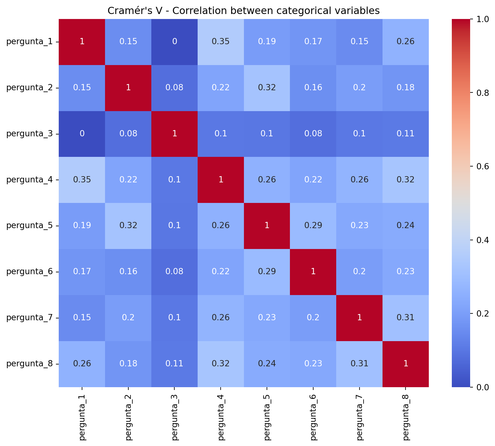
Visualizing the correlation matrix:
Show Code
plt.figure(figsize=(10,8))sns.heatmap(cramers_results, annot=True, cmap='coolwarm', vmin=0, vmax=1)plt.title("Cramér's V - Correlation between categorical variables")plt.show()
We do not have highly correlated variables, but let’s analyze the three largest correlations to assess the consistency of this dataset.
Evaluating the three largest correlations:
Show Code
# Transformar a matriz em long format (par variável - valor de correlação)corr_pairs = ( cramers_results.where(np.triu(np.ones(cramers_results.shape), k=1).astype(bool)) # pegar só triângulo superior (evita repetição) .stack() # transformar em Series com MultiIndex .reset_index())corr_pairs.columns = ['1', '2', 'Cramers_V']# Ordenar pelas maiores correlaçõestop_corr = corr_pairs.sort_values(by='Cramers_V', ascending=False).head(3)print(top_corr)
('Nível de clareza sobre o casamento dos sonhos: Como vocês descreveriam o nível de clareza que têm sobre o casamento que desejam?',
 'Nível de organização do planejamento: Como vocês estão se organizando para planejar o casamento?')
This correlation makes sense because those who have clarity about the wedding they desire tend to be more organized regarding the planning.
('Nível de organização do planejamento: Como vocês estão se organizando para planejar o casamento?',
 'Comprometimento em tornar esse sonho realidade: O quanto vocês estão comprometidos em transformar esse sonho em realidade?')
This correlation also makes sense because those who are more organized will be more committed to making the wedding happen.
('Situação financeira atual: Como você descreveria a situação financeira atual de vocês dois?',
 'Possibilidade de investimento atual no casamento: Se fossem realizar o casamento ideal hoje, como pagariam?')
These questions also have a justifiable correlation, as the couple’s financial situation will directly impact the possibility of current investment in the wedding
Conclusion
There are no very strong relationships between the questions, which is expected in well-designed questionnaires where questions measure distinct, albeit related, aspects (no high risk of multicollinearity).
The highest correlations are classified as moderate or weak, indicating that each question captures different aspects of the leads’ profile or situation.
We will still apply PCA for dimensionality reduction, but it is not mandatory due to multicollinearity between variables, but rather because we are interested in reducing computational complexity and improving the efficiency of KNN in high-dimensional spaces.
One-Hot-Encoding Application
Since we have many features and need to feed the algorithm with numerical variables, we will apply OHE with the drop_first=True parameter. OHE transforms categorical variables into a binary numerical format, essential for algorithms that do not natively handle categories, as is the case with KMeans.
Applying One-Hot Encoding with drop_first=True:
Show Code
# Instanciando o codificadorohe = OneHotEncoder(drop='first', sparse=False)# Ajustando e transformando os dadosohe_array = ohe.fit_transform(df_gf)# Pegando os nomes das colunas geradas pelo OHEohe_columns = ohe.get_feature_names_out(df_gf.columns)# Criando um novo DataFrame com os dados codificadosdf_gf_ohe = pd.DataFrame(ohe_array, columns=ohe_columns, index=df_gf.index)# Visualizando amostra aleatória de 10 linhasdf_gf_ohe.sample(10)
pergunta_1_B
pergunta_1_C
pergunta_1_D
pergunta_2_B
pergunta_2_C
pergunta_2_D
pergunta_3_B
pergunta_3_C
pergunta_3_D
pergunta_4_B
...
pergunta_5_D
pergunta_6_B
pergunta_6_C
pergunta_6_D
pergunta_7_B
pergunta_7_C
pergunta_7_D
pergunta_8_B
pergunta_8_C
pergunta_8_D
606
0.0
0.0
0.0
0.0
0.0
0.0
0.0
0.0
0.0
0.0
...
0.0
0.0
0.0
0.0
0.0
0.0
0.0
0.0
0.0
0.0
222
0.0
0.0
1.0
0.0
0.0
0.0
1.0
0.0
0.0
0.0
...
0.0
0.0
1.0
0.0
0.0
0.0
0.0
0.0
1.0
0.0
160
0.0
0.0
0.0
0.0
1.0
0.0
0.0
0.0
0.0
0.0
...
0.0
1.0
0.0
0.0
0.0
1.0
0.0
0.0
1.0
0.0
287
0.0
1.0
0.0
1.0
0.0
0.0
0.0
0.0
0.0
0.0
...
0.0
1.0
0.0
0.0
0.0
0.0
0.0
1.0
0.0
0.0
393
1.0
0.0
0.0
0.0
0.0
0.0
0.0
0.0
0.0
0.0
...
0.0
1.0
0.0
0.0
0.0
0.0
0.0
1.0
0.0
0.0
566
0.0
1.0
0.0
1.0
0.0
0.0
0.0
0.0
0.0
1.0
...
0.0
1.0
0.0
0.0
0.0
0.0
0.0
1.0
0.0
0.0
602
0.0
1.0
0.0
0.0
0.0
0.0
0.0
0.0
0.0
1.0
...
0.0
1.0
0.0
0.0
1.0
0.0
0.0
0.0
0.0
1.0
593
0.0
0.0
0.0
1.0
0.0
0.0
1.0
0.0
0.0
0.0
...
0.0
1.0
0.0
0.0
0.0
0.0
0.0
0.0
0.0
0.0
227
1.0
0.0
0.0
1.0
0.0
0.0
0.0
0.0
0.0
1.0
...
0.0
1.0
0.0
0.0
0.0
0.0
0.0
0.0
0.0
0.0
463
0.0
0.0
0.0
0.0
0.0
0.0
0.0
0.0
0.0
0.0
...
0.0
0.0
0.0
0.0
0.0
0.0
0.0
0.0
1.0
0.0
10 rows × 24 columns
We can see the use of the drop=‘first’ parameter, which removes the first category of each variable to reduce dimensionality; we have 24 features instead of 32.
PCA Application
Principal Component Analysis (PCA) is a statistical dimensionality reduction technique that transforms a set of possibly correlated variables into a new set of uncorrelated variables, called principal components.
The objective for our project is to capture the maximum variability of the data in the first components and facilitate visualization, clustering, classification, and reduce noise. OHE significantly increases dimensionality (in this project’s case, from 8 questions to 24 variables after drop_first=True).
Applying PCA
Show Code
# Padronizando os dadosscaler = StandardScaler()df_scaled = scaler.fit_transform(df_gf_ohe)# Instanciando o PCApca = PCA()# Ajustando o PCA aos dadospca.fit(df_scaled)# Gerando os componentes principaisdf_pca = pca.transform(df_scaled)# Convertendo em DataFrame para visualizaçãodf_pca = pd.DataFrame(df_pca, columns=[f'PC{i+1}'for i inrange(df_pca.shape[1])])# Visualizando as 5 primeiras linhasprint(df_pca.head())
The result of the principal component analysis aims to provide a basis for us to decide how many variables we will use and how much total variance we can explain in this dataset. Therefore, we should choose between 01 to 24 PCs and make a decision based on “how much we want to explain from this data,” i.e., the minimum components needed to have maximum interpretability.
Scree Plot - Explained Variance by PCA:
Show Code
# Dados da variância explicadavariancia_acumulada = np.cumsum(pca.explained_variance_ratio_)# Criando a figurafig = go.Figure()fig.add_trace( go.Scatter( x=list(range(1, len(variancia_acumulada) +1)), y=variancia_acumulada, mode='lines+markers', line=dict(dash='dash', width=2), marker=dict(size=8, color='blue'), name='Accumulated Variance' ))fig.update_layout( title='Scree Plot - Explained Variance by PCA', xaxis_title='Number of Components', yaxis_title='Accumulated Explained Variance', template='plotly_white', width=800, height=500)fig.show()
Visualizing the explained variance by each component:
Show Code
for i, var inenumerate(pca.explained_variance_ratio_):print(f'PC{i+1}: {var:.4f} ({np.cumsum(pca.explained_variance_ratio_)[i]:.4f} accumulated)')
We chose to use 17 principal components, which preserve 90.31% of the total variance of the dataset, ensuring a balance between data simplification and information maintenance. This value was determined based on the analysis of the scree plot and the accumulated variance distribution, which shows the absence of a clear elbow, characteristic of categorical data. This strategy allows for faster processing, improved model performance, and maintained analytical robustness.
Defining the Value of K in Clustering Models
The KMeans algorithm is a data clustering technique that organizes a set of points into groups (or “clusters”) based on their similarities. Choosing the appropriate value of k is an important step in the project, as it can significantly affect the usefulness of the formed clusters. To do this, we will use the Elbow Method and the Silhouette Score to help define an optimal value for k.
inertia = []K_range =range(1, 11)for k in K_range: kmeans = KMeans(n_clusters=k, random_state=42) kmeans.fit(df_pca) inertia.append(kmeans.inertia_)# Plot do Elbowfig = go.Figure()fig.add_trace( go.Scatter( x=list(K_range), y=inertia, mode='lines+markers', marker=dict(size=8, color='blue'), line=dict(width=2), name='Inertia' ))fig.update_layout( title='Elbow Method', xaxis_title='Number of Clusters (K)', yaxis_title='Inertia', template='plotly_white', width=800, height=500)fig.show()
Interpretation: evaluates the sum of squared distances within clusters (Sum of Squared Errors - SSE) as a function of different k values. As k increases, the error decreases, as the clusters become smaller and more specific. In the SSE vs. k graph, we look for the point where there is a “break” or “bend” (an elbow). This point indicates that increasing k beyond it brings marginal gains in error reduction, signaling the optimal number of clusters.
We can see where the curve forms an elbow between values 2 and 3, with k=2 being slightly more accentuated in its curvature, suggesting the best value for K, but it’s not very distinct for k=3.
Interpretation: The values measure the quality of clusters by calculating how similar a point is to its own cluster compared to other clusters. The value ranges between -1 (poor grouping) and 1 (optimal grouping). Here we can visualize the best value for k=3, but very close for k=2.
Results and Decision
Elbow Method - K = 2 The elbow shows where the reduction in inertia begins to stabilize.
Practical interpretation: The data may have two macro structures, meaning a coarser division.
Silhouette - Best at K = 3 The highest silhouette value (0.1239) occurs with K=3.
We will use k=2 and k=3 and analyze which algorithm best suits our project.
Applying KMeans Algorithm for K=2 and K=3:
Show Code
# Aplicar KMeans para k=2kmeans_k2 = KMeans(n_clusters=2, random_state=42)clusters_k2 = kmeans_k2.fit_predict(df_pca)# DataFrame com clusters K=2df_clusters_k2 = pd.DataFrame(df_pca, columns=[f'PC{i+1}'for i inrange(df_pca.shape[1])])df_clusters_k2['Cluster'] = clusters_k2# Aplicar KMeans para K=3kmeans_k3 = KMeans(n_clusters=3, random_state=42)clusters_k3 = kmeans_k3.fit_predict(df_pca)# DataFrame com clusters K=3df_clusters_k3 = pd.DataFrame(df_pca, columns=[f'PC{i+1}'for i inrange(df_pca.shape[1])])df_clusters_k3['Cluster'] = clusters_k3
Quantitative Evaluation of the two models – Silhouette Score:
## Distribuição dos Clustersprint("\nCluster Distribution - K=2")print(pd.Series(clusters_k2).value_counts())print("\nCluster Distribution - K=3")print(pd.Series(clusters_k3).value_counts())
Although the Silhouette metric is only slightly superior for K=3 (0.1239) compared to K=2 (0.1198), it still suggests that the model with three clusters offers a more refined division of respondents’ behavioral profiles.
The 2D PCA plots show some overlap between clusters (consistent with low silhouette scores) but also reveal that the cluster centers are in distinct positions, indicating that K-Means successfully found different patterns and that the groups capture relevant differences in behavioral profiles.
Based on the analysis of the centroids, which represent the average values (choice proportions) of each answer within each cluster, we can interpret that:
The closer to 1, the more predominant this characteristic is in the group.
Each value ranges from 0 to 1 and represents the relative frequency with which that option was chosen within the cluster.
This method allows us to understand the average profile and priorities of each segment.
Cluster Interpretation
Group 1: 234 leads (Cluster 1 — 47%)
Profile:
Wedding Style (Question 6): Predominantly, they desire “Something intimate and simple, only with close people” (🔸 pergunta_6_B – 99.6%). This is the most striking trait of this group.
Investment Possibility (Question 5): Most believe they “Could do something simple” if they were to have the wedding today (🔸 pergunta_5_B – 62.4%).
Organization Level (Question 4): A significant portion “Haven’t started yet” planning (🔸 pergunta_4_A – 57.3%).
Honeymoon Planning (Question 7): Most “Haven’t thought about it yet” (🔸 pergunta_7_A – 56.8%).
Partner’s Support (Question 3): The partner is “Completely involved, dreaming with me” (🔸 pergunta_3_A – 51.7%).
Behavior Summary:
This is the largest group and is characterized by a clear desire for a simpler, more intimate wedding.
Financially, they feel capable of holding a modest event, but have not yet started practical organization or honeymoon planning.
Partner involvement is high, indicating a shared dream.
Despite the desired simplicity, the lack of initiation in planning suggests a need for guidance to take the first steps, even for a smaller event.
Needs:
Ideas and inspirations for simple, elegant, and economical weddings.
Planning tools focused on smaller, more objective events.
Direction on how to start planning an intimate wedding without complications.
Content that validates the choice for a smaller wedding, showing its benefits and charm.
Group 2: 206 leads (Cluster 0 - 42%)
Profile:
Wedding Style (Question 6): They desire “A charming ceremony, with everything well done”, but not necessarily the most luxurious (🔸 pergunta_6_C – 62.6%).
Partner’s Support (Question 3): The partner is “Completely involved, dreaming with me” (🔸 pergunta_3_A – 53.4%).
Honeymoon Planning (Question 7): The vast majority “Haven’t thought about it yet” (🔸 pergunta_7_A – 49.0%).
Investment Possibility (Question 5): They feel they “Couldn’t afford anything yet” if the wedding were today (🔸 pergunta_5_A – 46.1%).
Organization Level (Question 4): They “Haven’t started yet” planning (🔸 pergunta_4_A – 44.7%).
Behavior Summary:
This group, one of the largest, is at a very early stage. They have clear dreams and desires about the ceremony style and have strong mutual support as a couple.
However, they face practical paralysis due to lack of organization and, crucially, the perception of financial incapacity at the moment.
They are dreaming big, but feel lost about where to start, with budget and organization being the main bottlenecks.
Needs:
Practical, step-by-step guides: “From scratch to dream wedding: a beginner’s guide”.
Solutions and ideas for affordable weddings: Content on how to achieve a charming ceremony on a limited budget.
Emotional and motivational content: Reinforcing that it’s normal to feel lost at the beginning and that it’s possible to turn the dream into reality with planning, even with limited resources.
Group 3: 55 leads (Cluster 2 — 11%)
Profile:
Clarity Level (Question 1): They have a very high level of clarity: “We know exactly what we want and have already started organizing” (�� pergunta_1_D – 89.1%).
Commitment (Question 8): They are highly committed: “We are ready, we want to act and truly achieve it” (🔸 pergunta_8_D – 85.5%).
Organization Level (Question 4): They are already well organized: “We have spreadsheets, goals, and even a defined timeline” (🔸 pergunta_4_D – 58.2%).
Investment Possibility (Question 5): They believe they “Could afford a good part, but we want more freedom” financially (🔸 pergunta_5_D – 49.1%).
Partner’s Support (Question 3): The partner is “Completely involved, dreaming with me” (🔸 pergunta_3_A – 47.3%).
Behavior Summary:
This is the smallest group, but it represents the most decisive and proactive brides.
They have total clarity about the desired wedding, are highly committed, and already have advanced planning.
Financially, they are in a relatively comfortable position, but seek to optimize their resources for “more freedom.”
Partner support is also strong, indicating a joint and aligned effort.
They have probably researched extensively and may be looking to optimize what they have already planned or find suppliers and solutions that fit their clear vision.
Needs:
Solutions to optimize the budget and maximize the value of the investment.
Advanced tools for vendor management or detailed timelines.
Specialized consulting to refine details or resolve specific planning points.
Inspiration for finishing touches or differentiated elements that add value to the already well-defined wedding.
Confirmation that they are on the right track and access to trusted suppliers.