Fitness Analytics Platform +LLM (End-to-End)

Author

Gabriel Ferreira

Published

February 12, 2026

Introduction

This project implements a complete end-to-end data engineering pipeline for strength training and nutrition data.

The objective was to design a production-style analytical data system capable of:

Auditing and validating raw operational data
Modeling relationally in PostgreSQL
Executing idempotent ETL pipelines
Producing deterministic weekly aggregations
Generating a canonical JSON contract for LLM consumption
Running in AWS under a controlled, low-cost architecture

Architecture Overview

graph TD
  A[Raw CSV: Hevy + Diet] --> B[Cleaning & Validation: Silver]
  B --> C[PostgreSQL: Normalized Schema]
  C --> D[Gold Weekly Views]
  D --> E[Canonical JSON Contract]
  E --> F[Amazon Bedrock: LLM Analysis]

The system was designed for deterministic weekly reproducibility.

Data Sources

Workout Data (Hevy)

Format: CSV export
Granularity: 1 row = 1 set
Historical coverage: 2023–2026
Total rows: 9542
Total unique exercises: 118

Diet Data

Source: SQLite (personal databse) → CSV export
Granularity: 1 row per day
Includes:
- Macros
- Calories
- Cardio volume
- Bodyweight
- Cycle classification

Stage 1: Raw Workout Data

Before modeling or automation, a full exploratory and quality audit was conducted.

Iinitial Load:

Show Code

df = pd.read_csv('hevy_workouts_raw.csv')
df.shape

(9542, 14)

Sample:

Show Code

df.head(10)

	title	start_time	end_time	description	exercise_title	superset_id	exercise_notes	set_index	set_type	weight_kg	reps	distance_km	duration_seconds	rpe
0	Lower	13 Jan 2026, 18:43	13 Jan 2026, 20:03	NaN	Hip Adduction (Machine)	NaN	NaN	0	normal	90.00	5.0	NaN	NaN	NaN
1	Lower	13 Jan 2026, 18:43	13 Jan 2026, 20:03	NaN	Hip Adduction (Machine)	NaN	NaN	1	normal	86.25	6.0	NaN	NaN	NaN
2	Lower	13 Jan 2026, 18:43	13 Jan 2026, 20:03	NaN	Hip Adduction (Machine)	NaN	NaN	2	failure	86.25	6.0	NaN	NaN	NaN
3	Lower	13 Jan 2026, 18:43	13 Jan 2026, 20:03	NaN	Straight Leg Deadlift	NaN	2RIR?	0	normal	100.00	6.0	NaN	NaN	NaN
4	Lower	13 Jan 2026, 18:43	13 Jan 2026, 20:03	NaN	Straight Leg Deadlift	NaN	2RIR?	1	normal	100.00	6.0	NaN	NaN	NaN
5	Lower	13 Jan 2026, 18:43	13 Jan 2026, 20:03	NaN	Leg Press (Machine)	NaN	2RIR	0	normal	260.00	5.0	NaN	NaN	NaN
6	Lower	13 Jan 2026, 18:43	13 Jan 2026, 20:03	NaN	Leg Press (Machine)	NaN	2RIR	1	normal	260.00	5.0	NaN	NaN	NaN
7	Lower	13 Jan 2026, 18:43	13 Jan 2026, 20:03	NaN	Seated Leg Curl (Machine)	NaN	NaN	0	normal	110.00	6.0	NaN	NaN	NaN
8	Lower	13 Jan 2026, 18:43	13 Jan 2026, 20:03	NaN	Leg Extension (Machine)	NaN	1RIR	0	normal	101.25	9.0	NaN	NaN	NaN
9	Lower	13 Jan 2026, 18:43	13 Jan 2026, 20:03	NaN	Leg Extension (Machine)	NaN	1RIR	1	normal	101.25	7.0	NaN	NaN	NaN

Types:

Show Code

df.dtypes

title                object
start_time           object
end_time             object
description          object
exercise_title       object
superset_id         float64
exercise_notes       object
set_index             int64
set_type             object
weight_kg           float64
reps                float64
distance_km         float64
duration_seconds    float64
rpe                 float64
dtype: object

Columns:

Show Code

df.columns

Index(['title', 'start_time', 'end_time', 'description', 'exercise_title',
       'superset_id', 'exercise_notes', 'set_index', 'set_type', 'weight_kg',
       'reps', 'distance_km', 'duration_seconds', 'rpe'],
      dtype='object')

There is no need to capture the training start and end times along with the date; therefore, we must split them into a column for the training date (training_date) and another for the training duration (derived from start_time and end_time).

EDA - Exploratory Data Analysis

Checking Missing Values:

Show Code

valores_ausentes = df.isnull().sum().sort_values(ascending = False)
print(valores_ausentes)

superset_id         9542
rpe                 9542
distance_km         9541
duration_seconds    9209
exercise_notes      8466
description         5264
weight_kg            708
reps                 333
title                  0
start_time             0
end_time               0
exercise_title         0
set_index              0
set_type               0
dtype: int64

superset_id: Never used; consistently contains null values.
rpe: Same status as superset_id (all values missing).
distance_km: Only applicable for treadmill workouts; usually null as I track by time.
duration_seconds: Cardio duration; only present in cardio exercises.
exercise_notes: Exercise-specific comments; optional/not always required.
description: Training session description added upon completion; also optional.
weight_kg: Null for bodyweight exercises and cardio (no load).
reps: To be analyzed.

weight_kg column missing values where ‘weight_kg’ is NaN and exercise type is not cardio:

Show Code

exercicios_excluidos = ['Treadmill', 'Stair Machine (Floors)', 'Stair Machine (Steps)', 'Stair Machine','Spinning', 'Walking', 'Air Bike']

linhas_ausentes_carga = df[
    df['weight_kg'].isna() &
    ~df['exercise_title'].isin(exercicios_excluidos)
]
linhas_ausentes_carga

	title	start_time	end_time	description	exercise_title	superset_id	exercise_notes	set_index	set_type	weight_kg	reps	distance_km	duration_seconds	rpe
1740	Upper I	26 May 2025, 19:46	26 May 2025, 21:23	NaN	Chest Dip (Assisted)	NaN	NaN	0	normal	NaN	8.0	NaN	NaN	NaN
1741	Upper I	26 May 2025, 19:46	26 May 2025, 21:23	NaN	Chest Dip (Assisted)	NaN	NaN	1	failure	NaN	8.0	NaN	NaN	NaN
1799	Upper I	19 May 2025, 19:54	19 May 2025, 21:43	NaN	Chest Dip (Assisted)	NaN	NaN	1	failure	NaN	7.0	NaN	NaN	NaN
3154	Push 2 e Pull 2	28 Dec 2024, 09:18	28 Dec 2024, 10:59	Pull 2	Romanian Chair Sit Ups	NaN	NaN	0	normal	NaN	9.0	NaN	NaN	NaN
3155	Push 2 e Pull 2	28 Dec 2024, 09:18	28 Dec 2024, 10:59	Pull 2	Romanian Chair Sit Ups	NaN	NaN	1	normal	NaN	7.0	NaN	NaN	NaN
...	...	...	...	...	...	...	...	...	...	...	...	...	...	...
9411	Treino A - Costas + Biceps	27 Nov 2023, 17:19	27 Nov 2023, 18:18	NaN	Back Extension (Hyperextension)	NaN	NaN	3	normal	NaN	10.0	NaN	NaN	NaN
9518	Treino A - Costas + Biceps	21 Nov 2023, 17:54	21 Nov 2023, 18:48	NaN	Back Extension (Hyperextension)	NaN	NaN	0	normal	NaN	10.0	NaN	NaN	NaN
9519	Treino A - Costas + Biceps	21 Nov 2023, 17:54	21 Nov 2023, 18:48	NaN	Back Extension (Hyperextension)	NaN	NaN	1	normal	NaN	10.0	NaN	NaN	NaN
9520	Treino A - Costas + Biceps	21 Nov 2023, 17:54	21 Nov 2023, 18:48	NaN	Back Extension (Hyperextension)	NaN	NaN	2	normal	NaN	10.0	NaN	NaN	NaN
9521	Treino A - Costas + Biceps	21 Nov 2023, 17:54	21 Nov 2023, 18:48	NaN	Back Extension (Hyperextension)	NaN	NaN	3	normal	NaN	10.0	NaN	NaN	NaN

376 rows × 14 columns

Visualizing missing value distribution:

Show Code

linhas_ausentes_carga = df[
    df['weight_kg'].isna() &
    ~df['exercise_title'].isin(exercicios_excluidos)
]
linhas_ausentes_carga['exercise_title'].value_counts()

exercise_title
Back Extension (Hyperextension)    201
Pull Up                             86
Knee Raise Parallel Bars            53
Leg Raise Parallel Bars              8
Bench Dip                            7
Decline Crunch                       4
Chin Up                              4
Chest Dip (Assisted)                 3
Romanian Chair Sit Ups               3
Decline Crunch (Weighted)            2
Squat (Smith Machine)                1
Push Up                              1
Squat (Bodyweight)                   1
Bicep Curl (Machine)                 1
Plank                                1
Name: count, dtype: int64

Missing values for Back Extension (Hyperextension), Pull Up, Knee Raise Parallel Bars, Leg Raise Parallel Bars, Bench Dip, Decline Crunch, Chin Up, Chest Dip (Assisted), Romanian Chair Sit Ups, Decline Crunch (Weighted), Squat (Bodyweight), Push Up, and Plank are expected as these are bodyweight exercises. However, Bicep Curl (Machine) should not have missing values, and Squat (Smith Machine) was likely a zero-load warm-up, but we will investigate further.

Filtering these two exercises with null values in weight_kg:

Show Code

exercicios_interesse = [
    'Squat (Smith Machine)',
    'Bicep Curl (Machine)'
]

df[
    df['weight_kg'].isna() &
    df['exercise_title'].isin(exercicios_interesse)
]

	title	start_time	end_time	description	exercise_title	superset_id	exercise_notes	set_index	set_type	weight_kg	reps	distance_km	duration_seconds	rpe
5270	Perna Completo	31 Jul 2024, 07:42	31 Jul 2024, 09:01	NaN	Squat (Smith Machine)	NaN	NaN	0	warmup	NaN	30.0	NaN	NaN	NaN
6644	Costas + Biceps + Lombar - Treino 2	14 May 2024, 11:11	14 May 2024, 12:36	NaN	Bicep Curl (Machine)	NaN	NaN	2	failure	NaN	9.0	NaN	NaN	NaN

We confirmed the Smith Machine was a warm-up, but there is likely an error in the bicep exercise, as it is a set to failure and the set_index is 2, meaning it is the third set of this exercise.

Analyzing exactly this exercise on this specific date:

Show Code

df[
    (df['title'] == 'Costas + Biceps + Lombar - Treino 2') &
    (df['exercise_title'] == 'Bicep Curl (Machine)') &
    (df['start_time'].str.contains('14 May 2024'))
]

	title	start_time	end_time	description	exercise_title	superset_id	exercise_notes	set_index	set_type	weight_kg	reps	distance_km	duration_seconds	rpe
6642	Costas + Biceps + Lombar - Treino 2	14 May 2024, 11:11	14 May 2024, 12:36	NaN	Bicep Curl (Machine)	NaN	NaN	0	normal	54.0	12.0	NaN	NaN	NaN
6643	Costas + Biceps + Lombar - Treino 2	14 May 2024, 11:11	14 May 2024, 12:36	NaN	Bicep Curl (Machine)	NaN	NaN	1	failure	54.0	10.0	NaN	NaN	NaN
6644	Costas + Biceps + Lombar - Treino 2	14 May 2024, 11:11	14 May 2024, 12:36	NaN	Bicep Curl (Machine)	NaN	NaN	2	failure	NaN	9.0	NaN	NaN	NaN

After analysis, we confirmed a manual entry error, resulting in the missing value; the correct value is 54.0 kg.

Imputing the correct value for this set:

Show Code

df.loc[6644, 'weight_kg'] = 54.0

reps column missing values where ‘reps’ is NaN and exercise type is not cardio:

Show Code

exercicios_excluidos = ['Treadmill', 'Stair Machine (Floors)', 'Stair Machine (Steps)', 'Stair Machine','Spinning', 'Walking', 'Air Bike']

linhas_ausentes_repeticoes = df[
    df['reps'].isna() &
    ~df['exercise_title'].isin(exercicios_excluidos)
]

linhas_ausentes_repeticoes

	title	start_time	end_time	description	exercise_title	superset_id	exercise_notes	set_index	set_type	weight_kg	reps	distance_km	duration_seconds	rpe
8022	(S1 ) Peito + Triceps + Abs - Treino 1	26 Feb 2024, 10:54	26 Feb 2024, 11:53	Treino 6	Plank	NaN	NaN	0	normal	NaN	NaN	NaN	48.0	NaN

Plank is also an exercise where the absence of repetitions is expected and acceptable

Outlier Detectition

Function to detect outliers using the IQR (Interquartile Range) method:

Show Code

def detectar_outliers(df, coluna):
    Q1 = df[coluna].quantile(0.25)
    Q3 = df[coluna].quantile(0.75)
    IQR = Q3 - Q1
    limite_inferior = Q1 - 1.5 * IQR
    limite_superior = Q3 + 1.5 * IQR
    
    outliers = df[(df[coluna] < limite_inferior) | (df[coluna] > limite_superior)]
    return outliers

Detecting and displaying total outliers per column:

Show Code

colunas = ['weight_kg', 'reps']
for coluna in colunas:
    outliers = detectar_outliers(df, coluna)
    print(f"Total de outliers em '{coluna}': {len(outliers)}")

Total de outliers em 'weight_kg': 121
Total de outliers em 'reps': 239

Detect and display outliers for the ‘weight_kg’ column:

Show Code

outliers_carga_kg = detectar_outliers(df, 'weight_kg')

if not outliers_carga_kg.empty:
    print("Outliers em 'weight_kg (119) ':")
    print(outliers_carga_kg[['exercise_title', 'start_time', 'weight_kg', 'reps']])

Outliers em 'weight_kg (119) ':
           exercise_title          start_time  weight_kg  reps
5     Leg Press (Machine)  13 Jan 2026, 18:43      260.0   5.0
6     Leg Press (Machine)  13 Jan 2026, 18:43      260.0   5.0
73    Leg Press (Machine)   6 Jan 2026, 19:46      280.0   6.0
74    Leg Press (Machine)   6 Jan 2026, 19:46      280.0   5.0
132   Leg Press (Machine)  30 Dec 2025, 18:26      280.0   5.0
133   Leg Press (Machine)  30 Dec 2025, 18:26      260.0   6.0
186   Leg Press (Machine)  23 Dec 2025, 11:58      280.0   7.0
187   Leg Press (Machine)  23 Dec 2025, 11:58      260.0   7.0
252   Leg Press (Machine)  16 Dec 2025, 19:47      280.0   7.0
253   Leg Press (Machine)  16 Dec 2025, 19:47      280.0   6.0
309   Leg Press (Machine)   9 Dec 2025, 20:32      280.0   7.0
310   Leg Press (Machine)   9 Dec 2025, 20:32      280.0   6.0
374   Leg Press (Machine)   2 Dec 2025, 20:03      280.0   6.0
375   Leg Press (Machine)   2 Dec 2025, 20:03      280.0   5.0
464   Leg Press (Machine)  18 Nov 2025, 19:25      275.0   6.0
465   Leg Press (Machine)  18 Nov 2025, 19:25      275.0   6.0
522   Leg Press (Machine)  11 Nov 2025, 20:13      270.0   7.0
523   Leg Press (Machine)  11 Nov 2025, 20:13      275.0   6.0
583   Leg Press (Machine)   4 Nov 2025, 20:10      270.0   7.0
584   Leg Press (Machine)   4 Nov 2025, 20:10      270.0   7.0
647   Leg Press (Machine)  28 Oct 2025, 19:41      270.0   7.0
648   Leg Press (Machine)  28 Oct 2025, 19:41      270.0   7.0
713   Leg Press (Machine)  21 Oct 2025, 19:50      270.0   6.0
714   Leg Press (Machine)  21 Oct 2025, 19:50      270.0   6.0
771   Leg Press (Machine)  14 Oct 2025, 19:57      265.0   7.0
772   Leg Press (Machine)  14 Oct 2025, 19:57      267.0   6.0
826   Leg Press (Machine)   7 Oct 2025, 20:24      265.0   7.0
827   Leg Press (Machine)   7 Oct 2025, 20:24      265.0   6.0
914   Leg Press (Machine)  23 Sep 2025, 19:21      265.0   6.0
915   Leg Press (Machine)  23 Sep 2025, 19:21      265.0   6.0
965   Leg Press (Machine)  16 Sep 2025, 19:37      265.0   6.0
966   Leg Press (Machine)  16 Sep 2025, 19:37      265.0   6.0
1022  Leg Press (Machine)   9 Sep 2025, 20:22      265.0   6.0
1023  Leg Press (Machine)   9 Sep 2025, 20:22      265.0   5.0
1081  Leg Press (Machine)   2 Sep 2025, 20:23      260.0   7.0
1082  Leg Press (Machine)   2 Sep 2025, 20:23      265.0   6.0
1136  Leg Press (Machine)  26 Aug 2025, 20:35      260.0   7.0
1137  Leg Press (Machine)  26 Aug 2025, 20:35      260.0   6.0
1236  Leg Press (Machine)  29 Jul 2025, 19:49      250.0   7.0
1237  Leg Press (Machine)  29 Jul 2025, 19:49      260.0   6.0
1554  Leg Press (Machine)  17 Jun 2025, 20:14      260.0   5.0
1555  Leg Press (Machine)  17 Jun 2025, 20:14      260.0   6.0
1613  Leg Press (Machine)  10 Jun 2025, 20:17      260.0   6.0
1614  Leg Press (Machine)  10 Jun 2025, 20:17      260.0   5.0
1671  Leg Press (Machine)   3 Jun 2025, 19:51      255.0   7.0
1672  Leg Press (Machine)   3 Jun 2025, 19:51      260.0   6.0
1729  Leg Press (Machine)  27 May 2025, 19:55      250.0   7.0
1730  Leg Press (Machine)  27 May 2025, 19:55      255.0   6.0
1787  Leg Press (Machine)  20 May 2025, 20:06      250.0   7.0
1788  Leg Press (Machine)  20 May 2025, 20:06      250.0   6.0
1847  Leg Press (Machine)  13 May 2025, 19:48      240.0   7.0
1848  Leg Press (Machine)  13 May 2025, 19:48      250.0   7.0
1905  Leg Press (Machine)   6 May 2025, 07:17      280.0   6.0
1906  Leg Press (Machine)   6 May 2025, 07:17      280.0   5.0
1961  Leg Press (Machine)  29 Apr 2025, 07:11      280.0   8.0
1962  Leg Press (Machine)  29 Apr 2025, 07:11      285.0   8.0
2036  Leg Press (Machine)  15 Apr 2025, 20:28      280.0   8.0
2037  Leg Press (Machine)  15 Apr 2025, 20:28      285.0   8.0
2096  Leg Press (Machine)   8 Apr 2025, 19:14      260.0   8.0
2097  Leg Press (Machine)   8 Apr 2025, 19:14      270.0   8.0
2158  Leg Press (Machine)   1 Apr 2025, 06:28      260.0   8.0
2159  Leg Press (Machine)   1 Apr 2025, 06:28      270.0   7.0
2222  Leg Press (Machine)  25 Mar 2025, 19:14      240.0   8.0
2223  Leg Press (Machine)  25 Mar 2025, 19:14      270.0   7.0
2288  Leg Press (Machine)  18 Mar 2025, 18:29      240.0   8.0
2289  Leg Press (Machine)  18 Mar 2025, 18:29      260.0   8.0
2330  Leg Press (Machine)  14 Mar 2025, 18:32      240.0   9.0
2331  Leg Press (Machine)  14 Mar 2025, 18:32      260.0   8.0
2332  Leg Press (Machine)  14 Mar 2025, 18:32      280.0   7.0
3776  Leg Press (Machine)  13 Nov 2024, 07:04      200.0  12.0
3777  Leg Press (Machine)  13 Nov 2024, 07:04      220.0  10.0
3778  Leg Press (Machine)  13 Nov 2024, 07:04      240.0   9.0
4002  Leg Press (Machine)  30 Oct 2024, 07:14      200.0  10.0
4003  Leg Press (Machine)  30 Oct 2024, 07:14      220.0  10.0
4004  Leg Press (Machine)  30 Oct 2024, 07:14      240.0   8.0
4206  Leg Press (Machine)  16 Oct 2024, 07:12      160.0  10.0
4207  Leg Press (Machine)  16 Oct 2024, 07:12      200.0  10.0
4208  Leg Press (Machine)  16 Oct 2024, 07:12      240.0   8.0
5520  Leg Press (Machine)  17 Jan 2024, 12:00      160.0  11.0
5521  Leg Press (Machine)  17 Jan 2024, 12:00      160.0  10.0
5522  Leg Press (Machine)  17 Jan 2024, 12:00      200.0  10.0
5523  Leg Press (Machine)  17 Jan 2024, 12:00      200.0  10.0
7692  Leg Press (Machine)  13 Mar 2024, 11:03      160.0  11.0
7693  Leg Press (Machine)  13 Mar 2024, 11:03      160.0  10.0
7694  Leg Press (Machine)  13 Mar 2024, 11:03      200.0  10.0
7695  Leg Press (Machine)  13 Mar 2024, 11:03      200.0  10.0
8190  Leg Press (Machine)  14 Feb 2024, 11:07      200.0  12.0
8191  Leg Press (Machine)  14 Feb 2024, 11:07      200.0  12.0
8192  Leg Press (Machine)  14 Feb 2024, 11:07      200.0  11.0
8428  Leg Press (Machine)  31 Jan 2024, 10:53      200.0  11.0
8429  Leg Press (Machine)  31 Jan 2024, 10:53      200.0  10.0
8430  Leg Press (Machine)  31 Jan 2024, 10:53      200.0  10.0
8431  Leg Press (Machine)  31 Jan 2024, 10:53      200.0  10.0
8566  Leg Press (Machine)  24 Jan 2024, 10:52      200.0  11.0
8567  Leg Press (Machine)  24 Jan 2024, 10:52      200.0  10.0
8568  Leg Press (Machine)  24 Jan 2024, 10:52      200.0  10.0
8569  Leg Press (Machine)  24 Jan 2024, 10:52      200.0  10.0
8792  Leg Press (Machine)   2 Jan 2024, 17:11      200.0  10.0
8793  Leg Press (Machine)   2 Jan 2024, 17:11      200.0  10.0
8794  Leg Press (Machine)   2 Jan 2024, 17:11      200.0  10.0
8795  Leg Press (Machine)   2 Jan 2024, 17:11      200.0  10.0
8871  Leg Press (Machine)  29 Dec 2023, 10:40      200.0  10.0
8872  Leg Press (Machine)  29 Dec 2023, 10:40      200.0  10.0
8873  Leg Press (Machine)  29 Dec 2023, 10:40      200.0  10.0
8874  Leg Press (Machine)  29 Dec 2023, 10:40      200.0  10.0
9057  Leg Press (Machine)  18 Dec 2023, 10:45      200.0  10.0
9058  Leg Press (Machine)  18 Dec 2023, 10:45      200.0  10.0
9059  Leg Press (Machine)  18 Dec 2023, 10:45      200.0  10.0
9060  Leg Press (Machine)  18 Dec 2023, 10:45      200.0  10.0
9140  Leg Press (Machine)  12 Dec 2023, 10:44      200.0  10.0
9141  Leg Press (Machine)  12 Dec 2023, 10:44      200.0  10.0
9142  Leg Press (Machine)  12 Dec 2023, 10:44      200.0  10.0
9143  Leg Press (Machine)  12 Dec 2023, 10:44      240.0   9.0
9250  Leg Press (Machine)   6 Dec 2023, 17:48      200.0  10.0
9251  Leg Press (Machine)   6 Dec 2023, 17:48      200.0  10.0
9252  Leg Press (Machine)   6 Dec 2023, 17:48      200.0  10.0
9253  Leg Press (Machine)   6 Dec 2023, 17:48      240.0   9.0
9464  Leg Press (Machine)  20 Nov 2023, 17:37      160.0  10.0
9465  Leg Press (Machine)  20 Nov 2023, 17:37      160.0  10.0
9466  Leg Press (Machine)  20 Nov 2023, 17:37      160.0  10.0
9467  Leg Press (Machine)  20 Nov 2023, 17:37      160.0  10.0

Groups and counts how many outliers there are by exercise title:

Show Code

# 1. Detecta todos os outliers novamente
outliers_original = detectar_outliers(df, 'weight_kg')
# 2. Agrupa e conta quantos outliers existem por título de exercício
contagem_outliers = outliers_original['exercise_title'].value_counts()
print("Distribuição de Outliers por Exercício:")
print(contagem_outliers)

Distribuição de Outliers por Exercício:
exercise_title
Leg Press (Machine)    121
Name: count, dtype: int64

Legpress is an exercise where the absolute weight is significantly higher compared to the other exercises but they are not necessarily outliers

Leg Press (Machine) visualization:

Show Code

exercise_name = "Leg Press (Machine)"
df_ex = df[df["exercise_title"] == exercise_name]
fig = px.box(df_ex,y="weight_kg",points="all",hover_data=["reps","set_index","set_type","rpe","start_time"],title=f"Weight Distribuiton — {exercise_name}")
fig.update_layout(yaxis_title="Weight",xaxis_title="",showlegend=False,height=600,width=900,title_x = 0.5)
fig.show()

Correct values. Since my training is based on progressive overload, it makes sense that values close to 280 kg have few records, as they represent the most recent loads lifted.

Detect and display outliers for the ‘reps’ column:

Show Code

outliers_repeticoes = detectar_outliers(df, 'reps')

if not outliers_repeticoes.empty:
    print("Outliers em 'repeticoes (209) ':")
    print(outliers_repeticoes[['exercise_title','weight_kg', 'reps']])

Outliers em 'repeticoes (209) ':
                       exercise_title  weight_kg  reps
3860    Standing Calf Raise (Machine)       20.0  30.0
3861    Standing Calf Raise (Machine)       40.0  25.0
3862    Standing Calf Raise (Machine)       60.0  20.0
3867    Standing Calf Raise (Machine)       40.0  24.0
3868    Standing Calf Raise (Machine)       20.0  30.0
...                               ...        ...   ...
8907   Incline Bench Press (Dumbbell)       17.5  20.0
8957  Seated Shoulder Press (Machine)       37.5  20.0
9021  Seated Shoulder Press (Machine)       37.5  20.0
9105  Seated Shoulder Press (Machine)       37.5  20.0
9282             Cable Fly Crossovers       10.0  16.0

[239 rows x 3 columns]

Group and count outliers per exercise title:

Show Code

outliers_original = detectar_outliers(df, 'reps')

# 2. Agrupa e conta quantos outliers existem por título de exercício
contagem_outliers = outliers_original['exercise_title'].value_counts()

print("Distribuição de Outliers por Exercício:")
print(contagem_outliers)

Distribuição de Outliers por Exercício:
exercise_title
Standing Calf Raise (Machine)               117
Incline Bench Press (Dumbbell)               18
Lateral Raise (Dumbbell)                     11
Calf Extension (Machine)                      8
Chest Fly (Machine)                           8
Triceps Rope Pushdown                         7
Single Arm Tricep Extension (Dumbbell)        6
Triceps Extension (Cable)                     6
Lat Pulldown (Cable)                          6
Crunch (Machine)                              5
Preacher Curl (Machine)                       4
Single Arm Lateral Raise (Cable)              4
Lateral Raise (Machine)                       4
Chest Press (Machine)                         4
Lat Pulldown (Machine)                        4
Iso-Lateral High Row (Machine)                4
Seated Cable Row - V Grip (Cable)             4
Seated Incline Curl (Dumbbell)                3
Seated Shoulder Press (Machine)               3
Seated Wrist Extension (Barbell)              3
Bicep Curl (Dumbbell)                         3
Squat (Smith Machine)                         2
Seated Leg Curl (Machine)                     1
Single Leg Standing Calf Raise (Machine)      1
Back Extension (Machine)                      1
Single Arm Triceps Pushdown (Cable)           1
Cable Fly Crossovers                          1
Name: count, dtype: int64

Standing Calf Raise (Machine):

Show Code

exercise_name = "Standing Calf Raise (Machine)"
df_ex = df[df["exercise_title"] == exercise_name]
fig = px.box(df_ex,y="reps",points="all",hover_data=["reps","weight_kg","set_index","set_type","rpe","start_time"],title=f"Reps Distribuiton — {exercise_name}")
fig.update_layout(yaxis_title="Reps",xaxis_title="",showlegend=False,height=600,width=900,title_x = 0.5)
fig.show()

We evaluated all exercises flagged as outliers and the majority (as seen in the example above) were warm-up sets where no load or a very low load was used; therefore, they do not qualify as incorrect data. The only exception was the Preacher Curl (Machine), detailed below, which indeed contained a manual entry error in the number of repetitions and was handled separately.

Preacher Curl (Machine):

Show Code

exercise_name = "Preacher Curl (Machine)"
df_ex = df[df["exercise_title"] == exercise_name]
fig = px.box(df_ex,y="reps",points="all",hover_data=["reps","weight_kg","set_index","set_type","rpe","start_time"],title=f"Reps Distribuiton — {exercise_name}")
fig.update_layout(yaxis_title="Reps",xaxis_title="",showlegend=False,height=600,width=900,title_x = 0.5)
fig.show()

Here we have an incorrect value: where 111 is recorded, it should actually be 11 repetitions

Analyzing this specific exercise instance:

Show Code

df[
    (df['exercise_title'] == 'Preacher Curl (Machine)') &
    (df['start_time'].str.contains('23 Jan 2024'))
]

	title	start_time	end_time	description	exercise_title	superset_id	exercise_notes	set_index	set_type	weight_kg	reps	distance_km	duration_seconds	rpe
8604	Treino B - Costas + Biceps	23 Jan 2024, 11:09	23 Jan 2024, 12:09	NaN	Preacher Curl (Machine)	NaN	NaN	0	normal	48.75	12.0	NaN	NaN	NaN
8605	Treino B - Costas + Biceps	23 Jan 2024, 11:09	23 Jan 2024, 12:09	NaN	Preacher Curl (Machine)	NaN	NaN	1	normal	48.75	111.0	NaN	NaN	NaN
8606	Treino B - Costas + Biceps	23 Jan 2024, 11:09	23 Jan 2024, 12:09	NaN	Preacher Curl (Machine)	NaN	NaN	2	normal	48.75	12.0	NaN	NaN	NaN

Imputing the correct value for this set:

Show Code

df.loc[8605, 'reps'] = 11.0

Revalidating the corrected set:

Show Code

df[
    (df['exercise_title'] == 'Preacher Curl (Machine)') &
    (df['start_time'].str.contains('23 Jan 2024'))
]

	title	start_time	end_time	description	exercise_title	superset_id	exercise_notes	set_index	set_type	weight_kg	reps	distance_km	duration_seconds	rpe
8604	Treino B - Costas + Biceps	23 Jan 2024, 11:09	23 Jan 2024, 12:09	NaN	Preacher Curl (Machine)	NaN	NaN	0	normal	48.75	12.0	NaN	NaN	NaN
8605	Treino B - Costas + Biceps	23 Jan 2024, 11:09	23 Jan 2024, 12:09	NaN	Preacher Curl (Machine)	NaN	NaN	1	normal	48.75	11.0	NaN	NaN	NaN
8606	Treino B - Costas + Biceps	23 Jan 2024, 11:09	23 Jan 2024, 12:09	NaN	Preacher Curl (Machine)	NaN	NaN	2	normal	48.75	12.0	NaN	NaN	NaN

Validations

set_index:

Show Code

# Ordenando para garantir consistência
df_sorted = df.sort_values(
    by=["start_time", "exercise_title", "set_index"]
)

# Agrupando por treino + exercício
set_index_check = (
    df_sorted
    .groupby(["start_time", "exercise_title"])["set_index"]
    .apply(list)
    .reset_index(name="set_index_list")
)

# Funções de validação
def starts_with_zero(seq):
    return min(seq) == 0

def has_gaps(seq):
    return sorted(seq) != list(range(min(seq), max(seq) + 1))

# Aplicando validações
set_index_check["starts_with_zero"] = set_index_check["set_index_list"].apply(starts_with_zero)
set_index_check["has_gaps"] = set_index_check["set_index_list"].apply(has_gaps)

# Casos problemáticos
problemas_set_index = set_index_check[
    (~set_index_check["starts_with_zero"]) |
    (set_index_check["has_gaps"])
]

print(f"Total de exercícios analisados: {len(set_index_check)}")
print(f"Casos com problemas de set_index: {len(problemas_set_index)}")

problemas_set_index.head()

Total de exercícios analisados: 3447
Casos com problemas de set_index: 0

	start_time	exercise_title	set_index_list	starts_with_zero	has_gaps

Workout Duration:

Show Code

# Convertendo para datetime
df["start_time_dt"] = pd.to_datetime(df["start_time"], format="%d %b %Y, %H:%M")
df["end_time_dt"] = pd.to_datetime(df["end_time"], format="%d %b %Y, %H:%M")

# Calculando duração em minutos
df["duracao_treino_min"] = (
    (df["end_time_dt"] - df["start_time_dt"])
    .dt.total_seconds() / 60
)

# Agregando por treino (um treino pode ter várias linhas)
duracao_por_treino = (
    df.groupby(["title", "start_time"])
    .agg(
        duracao_min=("duracao_treino_min", "first")
    )
    .reset_index()
)

# Treinos muito longos (> 4 horas)
treinos_longos = duracao_por_treino[
    duracao_por_treino["duracao_min"] > 240
]

# Treinos muito curtos (< 10 minutos)
treinos_curtos = duracao_por_treino[
    duracao_por_treino["duracao_min"] < 10
]

print(f"Treinos > 4h: {len(treinos_longos)}")
print(f"Treinos < 10min: {len(treinos_curtos)}")

treinos_longos.head(), treinos_curtos.head()

Treinos > 4h: 0
Treinos < 10min: 0

(Empty DataFrame
 Columns: [title, start_time, duracao_min]
 Index: [],
 Empty DataFrame
 Columns: [title, start_time, duracao_min]
 Index: [])

Naming Consistency:

Show Code

# Total de exercícios únicos
exercicios_unicos = df["exercise_title"].nunique()

# Frequência por exercício
freq_exercicios = df["exercise_title"].value_counts()

# Exercícios que aparecem apenas 1 vez
exercicios_uma_vez = freq_exercicios[freq_exercicios == 1]

print(f"Total de exercícios únicos: {exercicios_unicos}")
print(f"Exercícios que aparecem apenas 1 vez: {len(exercicios_uma_vez)}")

exercicios_uma_vez.head(10)

Total de exercícios únicos: 118
Exercícios que aparecem apenas 1 vez: 5

exercise_title
Squat (Bodyweight)       1
Plank                    1
Push Up                  1
Walking                  1
Stair Machine (Steps)    1
Name: count, dtype: int64

Analysis

Workouts per day:

Show Code

# Treinos por dia
df["data_treino"] = df["start_time_dt"].dt.date

treinos_por_dia = (
    df.groupby("data_treino")["title"]
    .nunique()
    .reset_index(name="qtde_treinos")
)

fig = px.bar(
    treinos_por_dia,
    x="data_treino",
    y="qtde_treinos",
    title="Training Frequency Over Time"
)

fig.update_layout(
    xaxis_title="Data",
    yaxis_title="Workout Count",
    title_x=0.5,
    height=500
)

fig.show()

Load progression - Exercise: Seated Leg Curl (Machine):

Show Code

exercise_name = "Seated Leg Curl (Machine)"

df_ex = (
    df[df["exercise_title"] == exercise_name]
    .groupby("data_treino")
    .agg(carga_max=("weight_kg", "max"))
    .reset_index()
)

fig = px.line(
    df_ex,
    x="data_treino",
    y="carga_max",
    markers=True,
    title=f"Load progression — {exercise_name}"
)

fig.update_layout(
    xaxis_title="Data",
    yaxis_title="Maximum Weight (kg)",
    title_x=0.5,
    height=500
)

fig.show()

Load progression - Exercise: Chest Fly (Machine):

Show Code

exercise_name = "Chest Fly (Machine)"

df_ex = (
    df[df["exercise_title"] == exercise_name]
    .groupby("data_treino")
    .agg(carga_max=("weight_kg", "max"))
    .reset_index()
)

fig = px.line(
    df_ex,
    x="data_treino",
    y="carga_max",
    markers=True,
    title=f"Load progression — {exercise_name}"
)

fig.update_layout(
    xaxis_title="Data",
    yaxis_title="Maximum Weight (kg)",
    title_x=0.5,
    height=500
)

fig.show()

Scatter plot: weight vs. rep:

Show Code

fig = px.scatter(
    df,
    x="weight_kg",
    y="reps",
    color="set_type",
    opacity=0.6,
    title="Weight and Reps Scatter",
    hover_data=["exercise_title", "data_treino"]
)

fig.update_layout(
    xaxis_title="Wight (kg)",
    yaxis_title="Repetitions",
    title_x=0.5,
    height=600
)

fig.show()

Workout duration histogram:

Show Code

fig = px.histogram(
    duracao_por_treino,
    x="duracao_min",
    nbins=30,
    title="Workout Duration Distribution (min)"
)

fig.update_layout(
    xaxis_title="Duratiom (min)",
    yaxis_title="Train Count",
    title_x=0.5,
    height=500
)

fig.show()

Most frequent exercises:

Show Code

top_exercicios = (
    df["exercise_title"]
    .value_counts()
    .head(15)
    .reset_index()
)

top_exercicios.columns = ["exercise_title", "frequencia"]

fig = px.bar(
    top_exercicios,
    x="frequencia",
    y="exercise_title",
    orientation="h",
    title="Most Frequent Exercises (Top 15)"
)

fig.update_layout(
    xaxis_title="Number of sets",
    yaxis_title="",
    title_x=0.5,
    height=600,
    yaxis={'categoryorder':'total ascending'}
)

fig.show()

Set types (distribution):

Show Code

fig = px.pie(
    df,
    names="set_type",
    title="Set Type Distribution"
)

fig.update_layout(
    title_x=0.5,
    height=500
)

fig.show()

Training volume:

Show Code

# Garantindo a coluna de data
df["data_treino"] = df["start_time_dt"].dt.date

# Cada linha representa uma série → volume = contagem de linhas
volume_series_diario = (
    df.groupby("data_treino")
    .size()
    .reset_index(name="total_series")
)

fig = px.line(
    volume_series_diario,
    x="data_treino",
    y="total_series",
    markers=True,
    title="Trainning Volume per Day (Number of sets)"
)

fig.update_layout(
    xaxis_title="Data",
    yaxis_title="Total Sets",
    title_x=0.5,
    height=500
)

fig.show()

Set voulme by type:

Show Code

df["data_treino"] = df["start_time_dt"].dt.date

df_efetivas = df[df["set_type"].isin(["normal", "failure"])]

volume_por_tipo = (
    df_efetivas
    .groupby(["data_treino", "set_type"])
    .size()
    .reset_index(name="total_series")
)

fig = px.area(
    volume_por_tipo,
    x="data_treino",
    y="total_series",
    color="set_type",
    title="Total Sets per Type"
)

fig.update_layout(
    xaxis_title="Data",
    yaxis_title="Total Sets",
    title_x=0.5,
    height=500
)

fig.show()

Final Dataset Export (Silver Layer):

Show Code

df.to_csv("hevy_workouts_clean.csv",index=False,encoding="utf-8")

Stage 2: Raw Diet Data

Before integrating nutrition data into the relational model, a full validation and structural audit was performed on the exported dataset from my personal SQLite database.

The objective of this stage was to:

Validate structural integrity
Ensure domain consistency
Confirm macro–calorie coherence
Normalize cycle identification
Produce an immutable clean dataset for ingestion

Initial Load:

Show Code

pd.set_option("display.max_rows", 200)
pd.set_option("display.max_colwidth", None)
df = pd.read_csv("diet_daily_raw_export.csv")
df.head()

	data	carboidratos_g	proteinas_g	gorduras_g	kcal	cardio_semanal_min	cicle	peso_kg	observacoes
0	2023-05-06	250	190	85	2525	210	1Cutting I (01/05/2023 - 17/09/2023)	104.3	NaN
1	2023-05-07	250	190	85	2525	210	1Cutting I (01/05/2023 - 17/09/2023)	104.3	NaN
2	2023-05-08	250	190	85	2525	210	1Cutting I (01/05/2023 - 17/09/2023)	104.3	NaN
3	2023-05-09	250	190	85	2525	210	1Cutting I (01/05/2023 - 17/09/2023)	104.3	NaN
4	2023-05-10	250	190	85	2525	210	1Cutting I (01/05/2023 - 17/09/2023)	104.3	NaN

Shape:

Show Code

df.shape

(982, 9)

Structural Overview:

Show Code

df.info()

<class 'pandas.core.frame.DataFrame'>
RangeIndex: 982 entries, 0 to 981
Data columns (total 9 columns):
 #   Column              Non-Null Count  Dtype  
---  ------              --------------  -----  
 0   data                982 non-null    object 
 1   carboidratos_g      982 non-null    int64  
 2   proteinas_g         982 non-null    int64  
 3   gorduras_g          982 non-null    int64  
 4   kcal                982 non-null    int64  
 5   cardio_semanal_min  982 non-null    int64  
 6   cicle               982 non-null    object 
 7   peso_kg             982 non-null    float64
 8   observacoes         173 non-null    object 
dtypes: float64(1), int64(5), object(3)
memory usage: 69.2+ KB

Observations:

No missing values in numeric macro columns
observacoes is optional (notes field)
data initially loaded as object (string)
cicle stored as free-text categorical field

Granularity validation:

Show Code

df.duplicated(subset=["data"]).sum()

np.int64(0)

This confirms the dataset respects the intended grain:

1 row = 1 day

Date conversion:

Show Code

df["data"] = pd.to_datetime(df["data"], errors="coerce")
df[df["data"].isna()]

	data	carboidratos_g	proteinas_g	gorduras_g	kcal	cardio_semanal_min	cicle	peso_kg	observacoes

No invalid dates detected.

This confirms full temporal integrity.

Missing Values Audit:

Show Code

df.isna().sum()

data                    0
carboidratos_g          0
proteinas_g             0
gorduras_g              0
kcal                    0
cardio_semanal_min      0
cicle                   0
peso_kg                 0
observacoes           809
dtype: int64

All macro and calorie fields fully populated
observacoes contains null values (expected and acceptable)
No missing bodyweight records
No missing cycle classification
No unexpected structural gaps were found.

Domain Validations:

Negative Value Check:

Show Code

numeric_cols = [
    "carboidratos_g",
    "proteinas_g",
    "gorduras_g",
    "kcal",
    "cardio_semanal_min",
    "peso_kg"
]

(df[numeric_cols] < 0).sum()

carboidratos_g        0
proteinas_g           0
gorduras_g            0
kcal                  0
cardio_semanal_min    0
peso_kg               0
dtype: int64

All zero.

No invalid negative values exist in:

Macros
Calories
Weekly cardio
Bodyweight

Caloric Consistency Validation:

Calories were validated against macro-derived energy:

Carbs = 4 kcal/g
Protein = 4 kcal/g
Fat = 9 kcal/g

Show Code

df["kcal_estimado"] = (
    df["carboidratos_g"] * 4 +
    df["proteinas_g"] * 4 +
    df["gorduras_g"] * 9
)

df[["kcal", "kcal_estimado"]].head(10)

	kcal	kcal_estimado
0	2525	2525
1	2525	2525
2	2525	2525
3	2525	2525
4	2525	2525
5	2525	2525
6	2525	2525
7	2425	2425
8	2425	2425
9	2425	2425

Difference distribution:

Show Code

(df["kcal"] - df["kcal_estimado"]).abs().describe()

count    982.000000
mean       0.020367
std        0.638226
min        0.000000
25%        0.000000
50%        0.000000
75%        0.000000
max       20.000000
dtype: float64

Findings:

Mean deviation ≈ 0.02 kcal
Maximum deviation: 20 kcal
75% of records show zero difference

Cycle Normalization:

The cicle column contains descriptive strings combining:

Sequential cycle number
Strategy (Cutting, Bulking, Reverse, Maintenance)
Date range

Unique values::

Show Code

df["cicle"].unique()

array(['1Cutting I (01/05/2023 - 17/09/2023)',
       '2Reversa I (18/09/2023 - 29/10/2023)',
       '3Cutting II (30/10/2023 - 23/02/2024)',
       '4Reversa II (24/02/2024 - 22/03/2024)',
       '5Bulking I (23/03/2024 - 19/05/2024)',
       '6Cutting III (20/05/2024 - 28/09/2024)',
       '7Bulking II (28/10/2024 - 01/01/2025)',
       '8Cutting IV (02/01/2025 - 17/04/2025)',
       '9Manutenção I (18/04/2025 - 05/10/2025)',
       '10Cutting V (06/10/2025 - XX/XX/XXXX)'], dtype=object)

To normalize this for relational modeling, a deterministic mapping was created:

Cycle map:

Show Code

cycle_map = {
    "1Cutting I (01/05/2023 - 17/09/2023)": 1,
    "2Reversa I (18/09/2023 - 29/10/2023)": 2,
    "3Cutting II (30/10/2023 - 23/02/2024)": 3,
    "4Reversa II (24/02/2024 - 22/03/2024)": 4,
    "5Bulking I (23/03/2024 - 19/05/2024)": 5,
    "6Cutting III (20/05/2024 - 28/09/2024)": 6,
    "7Bulking II (28/10/2024 - 01/01/2025)": 7,
    "8Cutting IV (02/01/2025 - 17/04/2025)": 8,
    "9Manutenção I (18/04/2025 - 05/10/2025)": 9,
    "10Cutting V (06/10/2025 - XX/XX/XXXX)": 10
}

df["cycle_id"] = df["cicle"].map(cycle_map)
df[df["cycle_id"].isna()][["data", "cicle"]]

	data	cicle

Result:

No unmapped values.

This guarantees referential integrity for the future cycles dimension table.

Column Standardization:

Columns were renamed to follow the project’s naming conventions:

English
Snake case
Explicit semantic meaning

Show Code

df = df.rename(columns={
    "data": "diet_date",
    "carboidratos_g": "carbs_g",
    "proteinas_g": "protein_g",
    "gorduras_g": "fat_g",
    "kcal": "calories_kcal",
    "cardio_seamanal_min": "cardio_weekly_min",
    "peso_kg": "bodyweight_kg",
    "observacoes": "notes"
})
df = df.drop(columns=["cicle", "kcal_estimado"])
df = df.replace({np.nan: None})

Final Dataset Export (Silver Layer):

Show Code

df.to_csv(
    "diet_daily_clean.csv",
    index=False,
    encoding="utf-8"
)

Stage 3: Relational Modeling (Amazon RDS)

After validating and cleaning both training and nutrition datasets, the next step was the implementation of a normalized relational model.

This stage was executed in:

Amazon RDS — PostgreSQL (Managed Database Service)

The objective was to:

Move from flat CSV structure to normalized relational modeling
Enforce referential integrity
Guarantee deterministic aggregations
Enable performant weekly analytics
Prepare the system for idempotent ETL ingestion

Infrastructure Context

Database engine: PostgreSQL
Deployment: Amazon RDS
Schema: fitness
Connection: SSL-enabled

RDS was intentionally chosen to:

Simulate a production-style managed database
Avoid local-only architecture
Demonstrate cloud database provisioning
Keep operational overhead minimal

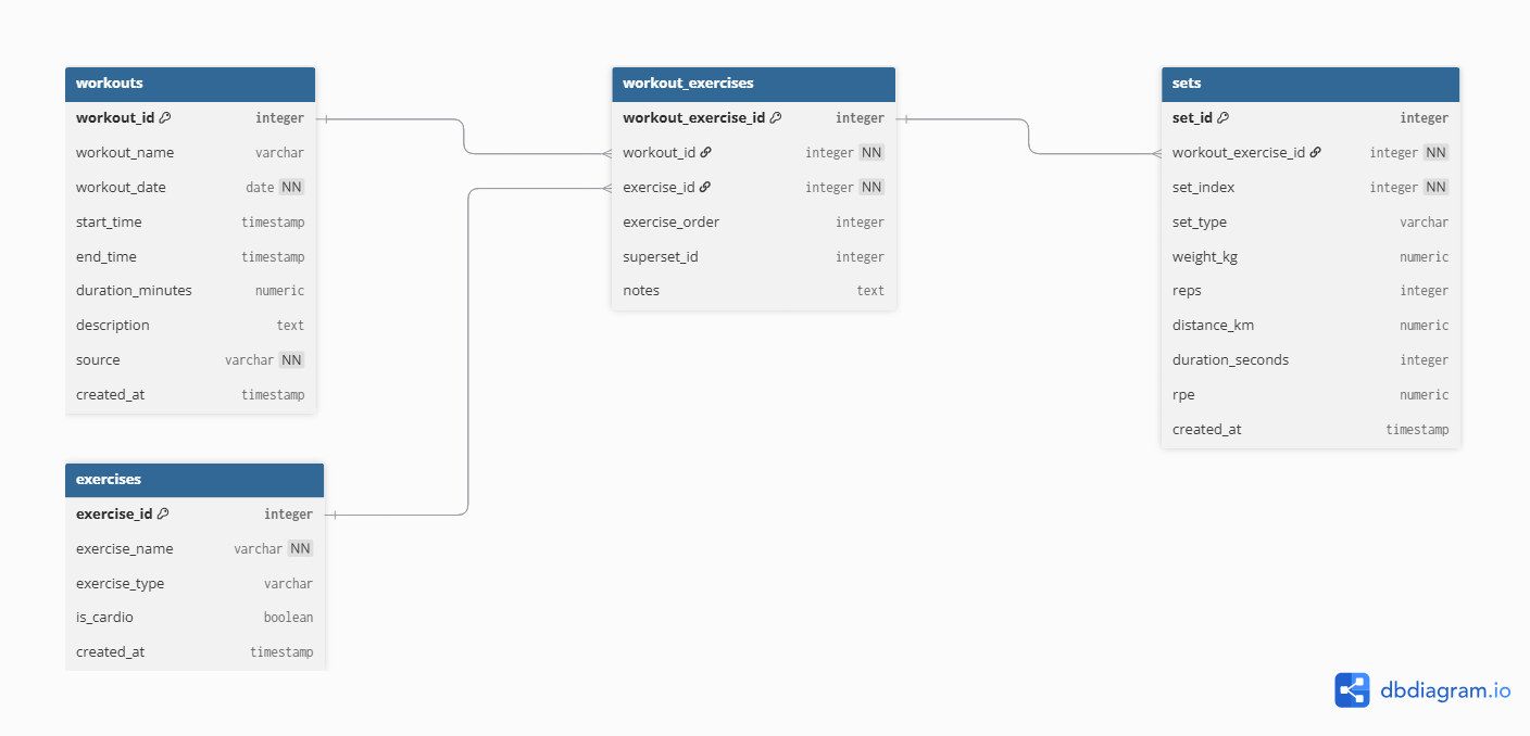
Database ER Diagram

Schema Definition

The schema was explicitly defined to isolate all project objects.

Show SQL

CREATE SCHEMA IF NOT EXISTS fitness;
SET search_path TO fitness;

This ensures:

Logical separation
Namespace clarity
Clean migration management

Core Tables

The modeling follows a normalized structure where:

1 workout → many exercises 1 exercise → many sets 1 day → 1 diet record

Foreign keys enforce consistency across all relationships.

Table: exercises

Show SQL

CREATE TABLE exercises (
    exercise_id SERIAL PRIMARY KEY,
    exercise_name TEXT NOT NULL UNIQUE,
    exercise_type TEXT,
    is_cardio BOOLEAN,
    created_at TIMESTAMP DEFAULT NOW()
);

Design Notes

exercise_name is UNIQUE to prevent duplication during ETL.
is_cardio allows future semantic filtering.
exercise_type reserved for future classification (not hardcoded yet).
Timestamp ensures traceability.

This table acts as a dimension table for exercises.

Table: workouts

Show SQL

CREATE TABLE workouts (
    workout_id SERIAL PRIMARY KEY,
    workout_name TEXT,
    workout_date DATE NOT NULL,
    start_time TIMESTAMP,
    end_time TIMESTAMP,
    duration_minutes NUMERIC(5,2),
    description TEXT,
    source TEXT NOT NULL,
    created_at TIMESTAMP DEFAULT NOW()
);

Design Notes

workout_date stored separately for aggregation performance.
duration_minutes precomputed to avoid runtime calculation overhead.
source explicitly tracks ingestion origin (e.g., hevy_csv).
Not enforcing uniqueness constraint intentionally — allows ingestion flexibility if future multi-source system is introduced.

This table represents the training session grain.

Table: workout_exercises

Show SQL

CREATE TABLE workout_exercises (
    workout_exercise_id SERIAL PRIMARY KEY,
    workout_id INT NOT NULL REFERENCES workouts(workout_id) ON DELETE CASCADE,
    exercise_id INT NOT NULL REFERENCES exercises(exercise_id),
    exercise_order INT,
    superset_id INT,
    notes TEXT
);

Design Notes

This is a bridge table resolving:

Many exercises per workout
Exercise order inside workout
Superset grouping

ON DELETE CASCADE ensures:

Deleting a workout automatically deletes dependent records.

This avoids orphan data.

Table: sets

Show SQL

CREATE TABLE sets (
    set_id SERIAL PRIMARY KEY,
    workout_exercise_id INT NOT NULL REFERENCES workout_exercises(workout_exercise_id) ON DELETE CASCADE,
    set_index INT NOT NULL,
    set_type TEXT,
    weight_kg NUMERIC(6,2),
    reps INT,
    distance_km NUMERIC(6,3),
    duration_seconds INT,
    rpe NUMERIC(3,1),
    created_at TIMESTAMP DEFAULT NOW()
);

Design Notes

This is the most granular fact table.

Grain:

1 row = 1 set

Key decisions:

Numeric precision defined explicitly
set_type not constrained via ENUM to allow ingestion flexibility
No derived metrics stored (volume, 1RM etc.)
RPE stored but not enforced

All analytical metrics will be calculated in Gold layer views.

Performance Indexes

Indexes were created to optimize common aggregation paths.

Show SQL

CREATE INDEX idx_workouts_date ON workouts(workout_date);
CREATE INDEX idx_exercises_name ON exercises(exercise_name);
CREATE INDEX idx_sets_type ON sets(set_type);
CREATE INDEX idx_sets_workout_exercise ON sets(workout_exercise_id);

Index Strategy

workout_date → weekly aggregations
exercise_name → lookup & joins
set_type → filtering warmups/failure sets
workout_exercise_id → join optimization

Indexes were added intentionally after understanding expected query patterns.

Nutrition Table

Show SQL

CREATE TABLE diet_daily (
    diet_date DATE PRIMARY KEY,
    carbs_g INT,
    protein_g INT,
    fat_g INT,
    calories_kcal INT,
    cardio_weekly_min INT,
    cycle_id INT
        REFERENCES cycles(cycle_id),
    bodyweight_kg NUMERIC(5,2),
    notes TEXT,
    created_at TIMESTAMP DEFAULT NOW()
);

Design Notes

Grain:

1 row = 1 day

Key decisions:

diet_date is PRIMARY KEY → prevents duplicates
cycle_id references a dimension table (cycles)
No macro-derived metrics stored
cardio_weekly_min kept at daily level for consistency with original structure

This table enables:

Weekly averages
Cycle segmentation
Cross-analysis with training

Referential Integrity Strategy

Foreign keys were enforced in:

workout_exercises → workouts
workout_exercises → exercises
sets → workout_exercises
diet_daily → cycles

This guarantees:

No orphan sets
No unmapped exercises
No diet record without valid cycle

The model prevents silent corruption.

Stage 4: ETL Pipeline (Amazon RDS)

After validating and cleaning the raw datasets, the next step was to load the data into a normalized relational schema deployed in Amazon RDS (PostgreSQL).

The ETL pipeline was executed against an Amazon RDS PostgreSQL instance under the fitness schema.

Environment Configuration

Database credentials were managed through environment variables to avoid hardcoding secrets.

Show Code

import os
from dotenv import load_dotenv

# Carrega o .env da raiz do projeto
load_dotenv()

DB_HOST = os.getenv("DB_HOST")
DB_PORT = os.getenv("DB_PORT", "5432")
DB_NAME = os.getenv("DB_NAME", "postgres")
DB_USER = os.getenv("DB_USER", "postgres")
DB_PASSWORD = os.getenv("DB_PASSWORD")
DB_SCHEMA = os.getenv("DB_SCHEMA", "fitness")

CSV_PATH = os.getenv("CSV_PATH")

This ensures:

Secure configuration
Easy migration between local and AWS environments
No credentials stored in version control

Database Engine (Amazon RDS Connection)

Show Code

from sqlalchemy import create_engine
from etl.config.settings import (
    DB_HOST, DB_PORT, DB_NAME,
    DB_USER, DB_PASSWORD, DB_SCHEMA
)

def get_engine():
    if not DB_PASSWORD:
        raise RuntimeError("DB_PASSWORD não foi carregada do .env")

    url = (
        f"postgresql+psycopg2://{DB_USER}:{DB_PASSWORD}"
        f"@{DB_HOST}:{DB_PORT}/{DB_NAME}"
    )

    engine = create_engine(
        url,
        connect_args={"options": f"-csearch_path={DB_SCHEMA}"}
    )

    return engine

This engine connects directly to:

Amazon RDS → PostgreSQL → fitness schema

Load Order Strategy

Because of foreign key dependencies, the loading order must respect relational integrity:

exercises
workouts
workout_exercises
sets

This guarantees:

No orphan records
Valid foreign keys
Controlled dependency resolution

Load — Exercises

Show Code

import pandas as pd
from sqlalchemy import text
from etl.utils.db import get_engine
from etl.config.settings import CSV_PATH


def load_exercises():
    engine = get_engine()

    # 1. Ler CSV (Bronze → memória)
    df = pd.read_csv(CSV_PATH)

    # 2. Extrair exercícios únicos
    exercises = (
        df["exercise_title"]
        .dropna()
        .drop_duplicates()
        .sort_values()
        .to_frame(name="exercise_name")
    )

    # 3. Inferir se é cardio
    cardio_mask = (
        df.groupby("exercise_title")[["distance_km", "duration_seconds"]]
        .apply(lambda x: x.notna().any().any())
    )

    exercises["is_cardio"] = (
        exercises["exercise_name"]
        .map(cardio_mask)
        .fillna(False)
    )

    # 4. Inserção idempotente
    insert_sql = text("""
        INSERT INTO exercises (exercise_name, is_cardio)
        VALUES (:exercise_name, :is_cardio)
        ON CONFLICT (exercise_name) DO NOTHING;
    """)

    with engine.begin() as conn:
        conn.execute(
            insert_sql,
            exercises.to_dict(orient="records")
        )

    print(f"[OK] {len(exercises)} exercises processed.")

Key logic:

Extract unique exercises from CSV
Infer is_cardio
Insert using ON CONFLICT DO NOTHING

Idempotent insert:

Show SQL

INSERT INTO exercises (exercise_name, is_cardio)
VALUES (:exercise_name, :is_cardio)
ON CONFLICT (exercise_name) DO NOTHING;

This ensures:

Safe re-runs
No duplication
Deterministic state in RDS

Load — Workouts:

Show Code

import pandas as pd
from sqlalchemy import text
from etl.utils.db import get_engine
from etl.config.settings import CSV_PATH


def load_workouts():
    engine = get_engine()

    # 1. Ler CSV
    df = pd.read_csv(CSV_PATH)

    # 2. Parse datas
    df["start_time"] = pd.to_datetime(df["start_time"])
    df["end_time"] = pd.to_datetime(df["end_time"])

    # 3. Agrupar por sessão de treino
    workouts = (
        df.groupby(["title", "start_time", "end_time"], as_index=False)
        .agg(
            workout_name=("title", "first"),
            description=("description", "first")
        )
    )

    # 4. Campos derivados
    workouts["workout_date"] = workouts["start_time"].dt.date
    workouts["duration_minutes"] = (
        (workouts["end_time"] - workouts["start_time"])
        .dt.total_seconds() / 60
    )
    workouts["source"] = "hevy_csv"

    # 5. SQLs
    select_sql = text("""
        SELECT workout_id
        FROM workouts
        WHERE workout_name = :workout_name
          AND start_time = :start_time
          AND end_time = :end_time
    """)

    insert_sql = text("""
        INSERT INTO workouts (
            workout_name,
            workout_date,
            start_time,
            end_time,
            duration_minutes,
            description,
            source
        )
        VALUES (
            :workout_name,
            :workout_date,
            :start_time,
            :end_time,
            :duration_minutes,
            :description,
            :source
        )
    """)

    inserted = 0

    with engine.begin() as conn:
        for _, row in workouts.iterrows():
            exists = conn.execute(
                select_sql,
                {
                    "workout_name": row["workout_name"],
                    "start_time": row["start_time"],
                    "end_time": row["end_time"],
                }
            ).fetchone()

            if exists:
                continue

            conn.execute(insert_sql, row.to_dict())
            inserted += 1

    print(f"[OK] {inserted} workouts inserted.")

Steps:

Group by session (title, start_time, end_time)
Derive:
- workout_date
- duration_minutes
- source

Existence check:

Show SQL

SELECT workout_id
FROM workouts
WHERE workout_name = :workout_name
  AND start_time = :start_time
  AND end_time = :end_time

Only inserts if not found.

This prevents duplicate training sessions on re-execution.

Load — Workout Exercises:

Show Code

import pandas as pd
from sqlalchemy import text
from etl.utils.db import get_engine
from etl.config.settings import CSV_PATH


def load_workout_exercises():
    engine = get_engine()

    # 1. Ler CSV
    df = pd.read_csv(CSV_PATH)

    # Parse datas
    df["start_time"] = pd.to_datetime(df["start_time"])
    df["end_time"] = pd.to_datetime(df["end_time"])

    # 2. Buscar mapeamento de workouts
    with engine.begin() as conn:
        workouts_map = {
            (row.workout_name, row.start_time, row.end_time): row.workout_id
            for row in conn.execute(text("""
                SELECT workout_id, workout_name, start_time, end_time
                FROM workouts
            """))
        }

        exercises_map = {
            row.exercise_name: row.exercise_id
            for row in conn.execute(text("""
                SELECT exercise_id, exercise_name
                FROM exercises
            """))
        }

    # 3. Gerar estrutura workout_exercises
    records = []
    seen = set()

    for (
        workout_name,
        start_time,
        end_time
    ), group in df.groupby(["title", "start_time", "end_time"]):

        workout_id = workouts_map.get((workout_name, start_time, end_time))
        if not workout_id:
            continue

        exercise_sequence = (
            group["exercise_title"]
            .drop_duplicates()
            .tolist()
        )

        for order, exercise_name in enumerate(exercise_sequence):
            exercise_id = exercises_map.get(exercise_name)
            if not exercise_id:
                continue

            superset_id = (
                group[group["exercise_title"] == exercise_name]["superset_id"]
                .dropna()
                .unique()
            )
            superset_id = int(superset_id[0]) if len(superset_id) > 0 else None

            key = (workout_id, exercise_id, order)
            if key in seen:
                continue
            seen.add(key)

            records.append({
                "workout_id": workout_id,
                "exercise_id": exercise_id,
                "exercise_order": order,
                "superset_id": superset_id,
                "notes": None
            })

    # 4. Inserção idempotente
    insert_sql = text("""
        INSERT INTO workout_exercises (
            workout_id,
            exercise_id,
            exercise_order,
            superset_id,
            notes
        )
        VALUES (
            :workout_id,
            :exercise_id,
            :exercise_order,
            :superset_id,
            :notes
        )
        ON CONFLICT DO NOTHING;
    """)

    with engine.begin() as conn:
        conn.execute(insert_sql, records)

    print(f"[OK] {len(records)} workout_exercises processed.")

Responsibilities:

Map workouts → exercises
Preserve exercise order
Preserve superset relationships

Idempotent logic:

Show SQL

INSERT INTO workout_exercises (...)
VALUES (...)
ON CONFLICT DO NOTHING;

Ensures safe replay.

Load — Sets (Most Granular Layer):

Show Code

import pandas as pd
from sqlalchemy import text
from etl.utils.db import get_engine
from etl.config.settings import CSV_PATH


def clean_nan(value):
    """
    Converte NaN do pandas para None (NULL no PostgreSQL)
    """
    if pd.isna(value):
        return None
    return value


def load_sets():
    engine = get_engine()

    # 1. Ler CSV
    df = pd.read_csv(CSV_PATH)

    # Parse datas
    df["start_time"] = pd.to_datetime(df["start_time"])
    df["end_time"] = pd.to_datetime(df["end_time"])

    # 2. Mapas auxiliares
    with engine.begin() as conn:
        workouts_map = {
            (row.workout_name, row.start_time, row.end_time): row.workout_id
            for row in conn.execute(text("""
                SELECT workout_id, workout_name, start_time, end_time
                FROM workouts
            """))
        }

        exercises_map = {
            row.exercise_name: row.exercise_id
            for row in conn.execute(text("""
                SELECT exercise_id, exercise_name
                FROM exercises
            """))
        }

        workout_ex_map = {
            (row.workout_id, row.exercise_id, row.exercise_order): row.workout_exercise_id
            for row in conn.execute(text("""
                SELECT workout_exercise_id, workout_id, exercise_id, exercise_order
                FROM workout_exercises
            """))
        }

    inserted = 0

    insert_sql = text("""
        INSERT INTO sets (
            workout_exercise_id,
            set_index,
            set_type,
            weight_kg,
            reps,
            distance_km,
            duration_seconds,
            rpe
        )
        VALUES (
            :workout_exercise_id,
            :set_index,
            :set_type,
            :weight_kg,
            :reps,
            :distance_km,
            :duration_seconds,
            :rpe
        )
    """)

    exists_sql = text("""
        SELECT 1
        FROM sets
        WHERE workout_exercise_id = :workout_exercise_id
          AND set_index = :set_index
    """)

    with engine.begin() as conn:
        for (
            workout_name,
            start_time,
            end_time
        ), group in df.groupby(["title", "start_time", "end_time"]):

            workout_id = workouts_map.get((workout_name, start_time, end_time))
            if not workout_id:
                continue

            # Ordem dos exercícios dentro do treino
            exercise_sequence = (
                group["exercise_title"]
                .drop_duplicates()
                .tolist()
            )

            exercise_order_map = {
                name: idx for idx, name in enumerate(exercise_sequence)
            }

            for _, row in group.iterrows():
                exercise_id = exercises_map.get(row["exercise_title"])
                if not exercise_id:
                    continue

                exercise_order = exercise_order_map.get(row["exercise_title"])
                workout_exercise_id = workout_ex_map.get(
                    (workout_id, exercise_id, exercise_order)
                )

                if not workout_exercise_id:
                    continue

                exists = conn.execute(
                    exists_sql,
                    {
                        "workout_exercise_id": workout_exercise_id,
                        "set_index": int(row["set_index"]),
                    }
                ).fetchone()

                if exists:
                    continue

                conn.execute(
                    insert_sql,
                    {
                        "workout_exercise_id": workout_exercise_id,
                        "set_index": int(row["set_index"]),
                        "set_type": row["set_type"],
                        "weight_kg": clean_nan(row["weight_kg"]),
                        "reps": clean_nan(row["reps"]),
                        "distance_km": clean_nan(row["distance_km"]),
                        "duration_seconds": clean_nan(row["duration_seconds"]),
                        "rpe": clean_nan(row["rpe"]),
                    }
                )

                inserted += 1

    print(f"[OK] {inserted} sets inserted.")

This is the most sensitive layer:

1 row = 1 set
Must match workout_exercise_id
Must avoid duplication

Before insertion:

Convert NaN → NULL (PostgreSQL compatible)

Existence check:

Show SQL

SELECT 1
FROM sets
WHERE workout_exercise_id = :workout_exercise_id
  AND set_index = :set_index

If exists → skip If not → insert

This makes the pipeline:

Fully idempotent at the lowest grain level

Pipeline Orchestration:

All steps were orchestrated through a single execution entrypoint:

Show Code

from etl.load.load_exercises import load_exercises
from etl.load.load_workouts import load_workouts
from etl.load.load_workout_exercises import load_workout_exercises
from etl.load.load_sets import load_sets


def run():
    print("=== ETL STARTED ===")

    load_exercises()
    load_workouts()
    load_workout_exercises()
    load_sets()

    print("=== ETL FINISHED ===")


if __name__ == "__main__":
    run()

This executed directly against:

Amazon RDS (PostgreSQL)

Idempotency Validation

The ETL pipeline was executed multiple times directly in Amazon RDS to validate replay safety and deterministic behavior. Across repeated executions, no duplicate exercises, workouts, or sets were created, and no referential integrity violations occurred. Row counts remained stable, confirming that the loading logic — including ON CONFLICT clauses and explicit existence checks — guarantees idempotent behavior and consistent state reconstruction.

This validates that the pipeline is replay-safe by design, meaning the same input dataset always produces the same relational state without unintended duplication or corruption.

Production Characteristics

The ETL architecture was intentionally designed with production principles in mind. The modular structure, explicit foreign key mapping, deterministic execution order, and SQLAlchemy-based connectivity ensure that the pipeline can be easily extended into scheduled batch jobs, containerized workflows, or orchestrated environments such as Lambda or Airflow.

At this stage, validated CSV datasets were transformed into a fully normalized relational schema in Amazon RDS using PostgreSQL, idempotent SQL patterns, and controlled schema management. The system is now structurally stable, cloud-portable, and prepared for analytical aggregation in the Gold layer and subsequent LLM contract generation.

Stage 5: Gold Layer

After loading the normalized relational model into Amazon RDS (PostgreSQL), the next step was to build the Gold Layer.

This layer was designed specifically for:

Weekly deterministic aggregation
Safe week-over-week comparison
Explicit metric semantics
No hidden calculations
LLM-ready consumption

All views were created directly inside the Amazon RDS instance under the fitness schema.

Weekly Training Summary

This view aggregates training metrics at the weekly level.

Show SQL

CREATE OR REPLACE VIEW gold_weekly_fitness_summary AS
WITH training_summary AS (
    SELECT
        DATE_TRUNC('week', w.workout_date)::date AS week_start,
        COUNT(DISTINCT w.workout_id)             AS training_sessions,
        COUNT(s.set_id)                          AS total_sets,
        COUNT(*) FILTER (WHERE s.set_type = 'failure') AS failure_sets,
        ROUND(AVG(s.reps), 2)                    AS avg_reps_per_set
    FROM workouts w
    JOIN workout_exercises we
        ON w.workout_id = we.workout_id
    JOIN sets s
        ON we.workout_exercise_id = s.workout_exercise_id
    WHERE s.set_type <> 'warmup'
    GROUP BY week_start
)
SELECT
    d.week_start,

    -- Diet
    d.avg_calories_kcal,
    d.avg_carbs_g,
    d.avg_protein_g,
    d.avg_fat_g,
    d.avg_bodyweight_kg,
    d.cardio_weekly_min,
    d.logged_days,

    -- Training
    t.training_sessions,
    t.total_sets,
    t.failure_sets,
    t.avg_reps_per_set,

    -- Cycle
    c.cycle_name,
    c.cycle_type
FROM gold_weekly_diet_summary d
LEFT JOIN training_summary t
    ON d.week_start = t.week_start
LEFT JOIN cycles c
    ON d.cycle_id = c.cycle_id;

Purpose

This creates a stable weekly anchor containing:

Diet averages
Training volume
Failure intensity
Active cycle

This becomes the high-level weekly context layer.

Weekly Training Detail (Per Exercise)

Show SQL

CREATE OR REPLACE VIEW gold_weekly_training_detail AS
SELECT
    DATE_TRUNC('week', w.workout_date)::date AS week_start,

    e.exercise_name,
    mg.muscle_group_name,

    COUNT(s.set_id)                          AS total_sets,
    ROUND(AVG(s.weight_kg), 2)               AS avg_weight_kg,
    ROUND(AVG(s.reps), 2)                    AS avg_reps,
    MAX(s.weight_kg)                         AS max_weight_kg,

    COUNT(*) FILTER (WHERE s.set_type = 'failure') AS failure_sets
FROM workouts w
JOIN workout_exercises we
    ON w.workout_id = we.workout_id
JOIN exercises e
    ON we.exercise_id = e.exercise_id
JOIN exercise_muscle_map emm
    ON e.exercise_id = emm.exercise_id
JOIN muscle_groups mg
    ON emm.muscle_group_id = mg.muscle_group_id
JOIN sets s
    ON we.workout_exercise_id = s.workout_exercise_id
WHERE s.set_type <> 'warmup'
GROUP BY
    week_start,
    e.exercise_name,
    mg.muscle_group_name;

Purpose

This view exposes:

Volume by exercise
Muscle group mapping
Average and maximum loads
Failure density

This enables:

Muscle-specific analysis
Volume allocation insights
Performance segmentation

Weekly Exercise Performance (Structured Metrics)

Show SQL

CREATE OR REPLACE VIEW gold_weekly_exercise_performance AS
SELECT
    DATE_TRUNC('week', w.workout_date)::date AS week_start,

    e.exercise_id,
    e.exercise_name,
    mg.muscle_group_name,

    COUNT(s.set_id) AS total_sets,

    COUNT(*) FILTER (
        WHERE s.set_type = 'failure'
    ) AS failure_sets,

    ROUND(AVG(s.reps), 2) AS avg_reps,

    ROUND(AVG(s.weight_kg), 2) AS avg_weight_kg,
    MAX(s.weight_kg)           AS max_weight_kg,

    SUM(s.reps) AS total_reps,

    COUNT(DISTINCT w.workout_id) AS sessions_count

FROM workouts w
JOIN workout_exercises we
    ON w.workout_id = we.workout_id
JOIN sets s
    ON we.workout_exercise_id = s.workout_exercise_id
JOIN exercises e
    ON we.exercise_id = e.exercise_id
JOIN exercise_muscle_map emm
    ON e.exercise_id = emm.exercise_id
JOIN muscle_groups mg
    ON emm.muscle_group_id = mg.muscle_group_id

WHERE s.set_type <> 'warmup'

GROUP BY
    week_start,
    e.exercise_id,
    e.exercise_name,
    mg.muscle_group_name;

Purpose

This is the LLM-facing metric layer.

It produces:

Explicit totals
Explicit averages
Explicit max loads
Explicit session count

No inferred metrics. No derived semantics. Only controlled aggregations.

Week-over-Week Progression

This view introduces temporal comparison using window functions.

Show SQL

CREATE OR REPLACE VIEW gold_weekly_exercise_progression AS
SELECT
    week_start,
    exercise_id,
    exercise_name,
    muscle_group_name,

    -- Current week metrics
    total_sets,
    total_reps,
    avg_reps,
    avg_weight_kg,
    max_weight_kg,
    failure_sets,
    sessions_count,

    -- Previous week metrics
    LAG(total_sets)      OVER w AS prev_total_sets,
    LAG(total_reps)      OVER w AS prev_total_reps,
    LAG(avg_reps)        OVER w AS prev_avg_reps,
    LAG(avg_weight_kg)   OVER w AS prev_avg_weight_kg,
    LAG(max_weight_kg)   OVER w AS prev_max_weight_kg,
    LAG(failure_sets)    OVER w AS prev_failure_sets,

    -- Deltas
    total_sets    - LAG(total_sets)    OVER w AS delta_total_sets,
    total_reps    - LAG(total_reps)    OVER w AS delta_total_reps,
    avg_reps      - LAG(avg_reps)      OVER w AS delta_avg_reps,
    avg_weight_kg - LAG(avg_weight_kg) OVER w AS delta_avg_weight_kg,
    max_weight_kg - LAG(max_weight_kg) OVER w AS delta_max_weight_kg,
    failure_sets  - LAG(failure_sets)  OVER w AS delta_failure_sets

FROM gold_weekly_exercise_performance
WINDOW w AS (
    PARTITION BY exercise_id
    ORDER BY week_start
);

Purpose

This enables:

Deterministic progression tracking
Explicit deltas
Safe LLM comparison

Instead of asking the LLM to compute differences, the database computes them deterministically.

Final LLM Context View

This is the final structured analytical contract inside RDS.

Show SQL

CREATE OR REPLACE VIEW gold_llm_weekly_exercise_context AS
SELECT
    p.week_start,

    -- Exercise identity
    p.exercise_id,
    p.exercise_name,
    p.muscle_group_name,

    -- Training (current week)
    p.total_sets,
    p.total_reps,
    p.avg_reps,
    p.avg_weight_kg,
    p.max_weight_kg,
    p.failure_sets,
    p.sessions_count,

    -- Training deltas (vs previous week)
    p.delta_total_sets,
    p.delta_total_reps,
    p.delta_avg_reps,
    p.delta_avg_weight_kg,
    p.delta_max_weight_kg,
    p.delta_failure_sets,

    -- Diet context (weekly)
    d.avg_calories_kcal,
    d.avg_carbs_g,
    d.avg_protein_g,
    d.avg_fat_g,
    d.cardio_weekly_min,
    d.avg_bodyweight_kg,
    d.logged_days,

    -- Cycle context
    c.cycle_id,
    c.cycle_name,
    c.cycle_type

FROM gold_weekly_exercise_progression p
LEFT JOIN gold_weekly_diet_summary d
    ON p.week_start = d.week_start
LEFT JOIN cycles c
    ON d.cycle_id = c.cycle_id;

Purpose

This is the final structured semantic layer consumed by the JSON extractor.

It merges:

Exercise performance
Progression metrics
Diet context
Cycle context

Into a single analytical surface.

Gold Layer Summary

The Gold Layer was fully implemented inside Amazon RDS using SQL views.

Stage 6: Canonical JSON (LLM)

After building the normalized relational model and the Gold analytical layer, the final step was to generate a canonical, deterministic JSON contract designed specifically for language model consumption.

The goal was not to simply serialize database rows, but to:

Eliminate relational complexity
Remove ambiguity
Provide explicit deltas (no inference required)
Deliver a schema-stable, versioned payload

This JSON acts as the single source of truth for LLM analysis.

Design Principles

The canonical contract was designed under the following constraints:

One file per week
Fully deterministic structure
Explicit weekly progression deltas
No derived metrics inside the LLM
No missing semantic context
Schema versioning support

Schema Definition (Versioned Contract)

The schema is explicitly defined and version-controlled:

Show Code

{
  "week_start": "YYYY-MM-DD",
  "cycle": {
    "cycle_id": "int",
    "cycle_name": "string",
    "cycle_type": "cutting | bulking | maintenance | reverse"
  },
  "diet": {
    "avg_calories_kcal": "number",
    "avg_carbs_g": "number",
    "avg_protein_g": "number",
    "avg_fat_g": "number",
    "cardio_weekly_min": "number",
    "avg_bodyweight_kg": "number",
    "logged_days": "int"
  },
  "training_overview": {
    "training_sessions": "int",
    "total_sets": "int",
    "failure_sets": "int",
    "avg_reps_per_set": "number"
  },
  "exercises": [
    {
      "exercise_id": "int",
      "exercise_name": "string",
      "muscle_group": "string",
      "current_week": { ... },
      "delta_vs_last_week": { ... }
    }
  ]
}

Payload Builder Implementation

The JSON is generated from Gold views using a dedicated extraction script.

Show Code

import json
import os
from datetime import date
from decimal import Decimal

from sqlalchemy import text
from etl.utils.db import get_engine

# ===============================
# CONFIG
# ===============================

OUTPUT_DIR = "llm/payloads"
SCHEMA_VERSION = "v1"


# ===============================
# UTILS
# ===============================

def json_safe(value):
    """
    Converte tipos não serializáveis (Decimal, date, datetime)
    para formatos compatíveis com JSON.
    """
    if isinstance(value, Decimal):
        return float(value)
    if hasattr(value, "isoformat"):
        return value.isoformat()
    return value


# ===============================
# FETCH FUNCTIONS
# ===============================

def fetch_weekly_summary(conn, week_start):
    sql = text("""
        SELECT *
        FROM gold_weekly_fitness_summary
        WHERE week_start = :week_start
    """)
    row = conn.execute(
        sql,
        {"week_start": week_start}
    ).mappings().fetchone()

    return dict(row) if row else None


def fetch_exercise_context(conn, week_start):
    sql = text("""
        SELECT *
        FROM gold_llm_weekly_exercise_context_v1
        WHERE week_start = :week_start
        ORDER BY exercise_name
    """)

    rows = conn.execute(
        sql,
        {"week_start": week_start}
    ).mappings().fetchall()

    return [dict(r) for r in rows]


# ===============================
# PAYLOAD BUILDER
# ===============================

def build_payload(week_start: str):
    engine = get_engine()

    with engine.begin() as conn:
        weekly = fetch_weekly_summary(conn, week_start)
        if not weekly:
            raise RuntimeError(
                f"No weekly summary found for week_start={week_start}"
            )

        exercises_raw = fetch_exercise_context(conn, week_start)
        if not exercises_raw:
            raise RuntimeError(
                f"No exercise context found for week_start={week_start}"
            )

    # -------------------------------
    # Exercises
    # -------------------------------
    exercises = []

    for r in exercises_raw:
        exercises.append({
            "exercise_id": r["exercise_id"],
            "exercise_name": r["exercise_name"],
            "muscle_group": r["muscle_group_name"],

            "current_week": {
                "total_sets": r["current_total_sets"],
                "total_reps": r["current_total_reps"],
                "avg_reps": json_safe(r["current_avg_reps"]),
                "avg_weight_kg": json_safe(r["current_avg_weight_kg"]),
                "max_weight_kg": json_safe(r["current_max_weight_kg"]),
                "failure_sets": r["current_failure_sets"],
                "sessions_count": r["current_sessions"]
            },

            "delta_vs_last_week": {
                "total_sets": r["delta_sets"],
                "total_reps": r["delta_reps"],
                "avg_reps": json_safe(r["delta_avg_reps"]),
                "avg_weight_kg": json_safe(r["delta_avg_weight_kg"]),
                "max_weight_kg": json_safe(r["delta_max_weight_kg"]),
                "failure_sets": r["delta_failure_sets"]
            }
        })

    # -------------------------------
    # Final payload
    # -------------------------------
    payload = {
        "schema_version": SCHEMA_VERSION,
        "generated_at": date.today().isoformat(),
        "week_start": weekly["week_start"].isoformat(),

        "cycle": {
            "cycle_name": weekly["cycle_name"],
            "cycle_type": weekly["cycle_type"]
        },

        "diet": {
            "avg_calories_kcal": json_safe(weekly["avg_calories_kcal"]),
            "avg_carbs_g": json_safe(weekly["avg_carbs_g"]),
            "avg_protein_g": json_safe(weekly["avg_protein_g"]),
            "avg_fat_g": json_safe(weekly["avg_fat_g"]),
            "cardio_weekly_min": weekly["cardio_weekly_min"],
            "avg_bodyweight_kg": json_safe(weekly["avg_bodyweight_kg"]),
            "logged_days": weekly["logged_days"]
        },

        "training_overview": {
            "training_sessions": weekly["training_sessions"],
            "total_sets": weekly["total_sets"],
            "failure_sets": weekly["failure_sets"],
            "avg_reps_per_set": json_safe(weekly["avg_reps_per_set"])
        },

        "exercises": exercises
    }

    return payload


# ===============================
# SAVE
# ===============================

def save_payload(payload):
    os.makedirs(OUTPUT_DIR, exist_ok=True)

    fname = f"weekly_fitness_context_{payload['week_start']}.json"
    path = os.path.join(OUTPUT_DIR, fname)

    with open(path, "w", encoding="utf-8") as f:
        json.dump(payload, f, ensure_ascii=False, indent=2)

    return path


# ===============================
# MAIN
# ===============================

if __name__ == "__main__":
    # Use uma semana que você sabe que existe no banco
    WEEK_START = "2026-01-05"

    payload = build_payload(WEEK_START)
    path = save_payload(payload)

    print(f"[OK] Weekly context generated: {path}")

Why This Structure Is LLM-Optimal

The JSON contract was intentionally designed to eliminate the most common failure modes observed when large language models consume structured data. Instead of requiring the model to infer joins, compute temporal comparisons, or aggregate metrics on the fly, all calculations are performed upstream in the Gold layer. The LLM receives a fully contextualized, semantically complete representation of the week.

There are no implicit relationships left to interpret, no derived metrics to calculate, and no schema ambiguity. Weekly deltas are explicitly provided, progression is already computed, and all nutritional and training context is embedded within the same document. As a result, the model operates purely as an analytical reasoning layer rather than a data transformation engine. This dramatically increases reliability, interpretability, and consistency of responses.

Deterministic Properties

For any given week_start, the system always produces the exact same output. The canonical JSON is generated from stable Gold views, using a fixed schema definition, explicit ordering rules, and deterministic delta calculations based on window functions. There is no stochastic logic in the data layer, no dynamic field generation, and no schema mutation.

Because the transformation pipeline is idempotent and the Gold layer is reproducible, the JSON payload becomes a replay-safe artifact. Running the extraction process multiple times for the same week will always result in an identical file. This deterministic behavior is critical for safe LLM interaction, auditing, version control, and long-term system stability.

Architectural Role

The JSON contract represents the formal boundary between structured analytical data and generative AI systems. Upstream of this boundary, the system is strictly relational, normalized, and governed by SQL logic inside Amazon RDS. Downstream of this boundary, the system becomes model-agnostic and cloud-portable.

Because the contract is independent of any specific model provider, it can be stored in S3, consumed by Amazon Bedrock, OpenAI models, or any future inference endpoint without requiring changes to the data layer. This separation of concerns ensures that the analytical infrastructure remains stable even as the AI layer evolves.

Stage 7: AWS Execution

After the relational modeling, Gold-layer aggregation, and canonical JSON generation were completed, the final stage of the project was executed entirely within the AWS ecosystem.

The weekly payload generated from Amazon RDS was uploaded to Amazon S3 and consumed directly through Amazon Bedrock. The LLM interaction occurred inside the AWS environment, ensuring that the structured data layer, storage layer, and inference layer remained cloud-native and internally integrated.

The inference process followed this flow:

Amazon RDS (Gold Views) → Canonical JSON Extraction → S3 Upload → Amazon Bedrock (LLM Inference) → Generated Weekly Performance Report

The prompt was manually defined inside the Bedrock playground, and the JSON payload was provided as structured context. The model was instructed to generate a deterministic weekly analytical report, focusing on progression, regression, diet alignment, fatigue signals, and performance insights — without inventing metrics or extrapolating beyond the provided contract.

The entire execution was recorded to demonstrate real AWS operation, including payload submission and model response generation.

AWS Run-Once Execution (Bedrock Inference)

To demonstrate full cloud integration, the final analytical stage of the project was executed entirely inside Amazon Web Services.

This execution followed a run-once model, intentionally designed to validate the architecture while maintaining strict cost control. The objective was not continuous deployment, but architectural proof of integration between:

Structured relational data (Amazon RDS)
Canonical analytical artifact (JSON)
Generative AI inference (Amazon Bedrock)

S3 Bucket Creation and Canonical Payload Upload

The first step of the cloud execution layer was the creation of an Amazon S3 bucket to store the canonical JSON contract generated from the Gold layer.

The recorded demonstration includes:

Creation of a dedicated S3 bucket
Proper configuration and region selection
Upload of the generated weekly JSON payload
Verification of the object structure inside AWS

This step establishes S3 as the formal storage boundary between deterministic data engineering outputs and AI consumption layers.

By uploading the JSON to S3, the architecture aligns with production-grade patterns where:

Analytical artifacts are versioned
Outputs are cloud-stored
Downstream services can consume structured data
The data platform remains decoupled from inference engines

The S3 object represents the finalized analytical state of a given week_start.

Amazon Bedrock Prompt Execution and LLM Report Generation

After the canonical JSON was available in AWS, the next step was inference execution inside Amazon Bedrock.

In the recorded demonstration:

The Amazon Bedrock Playground was opened
A Claude model was selected
The canonical JSON payload was inserted as structured context
A engineered analytical prompt was defined
The model generated a weekly performance report
The result was reviewed and validated against the structured input

The prompt was designed to:

Constrain reasoning strictly to provided data
Avoid external assumptions
Focus on progression and regression signals
Correlate diet and training metrics
Produce structured analytical insights rather than narrative speculation

The model operates purely as an analytical reasoning layer, not as a data transformation layer.

This confirms that the system successfully transitions from:

Relational Modeling (RDS) → Analytical Aggregation (Gold Layer) → Deterministic JSON Contract → Cloud Storage (S3) → Generative Analysis (Bedrock)

The execution was run-once to minimize cloud costs, but the architecture fully supports future automation through event-driven or scheduled orchestration.

Project Conclusion

This project demonstrates the full construction of an end-to-end analytical data platform, starting from raw operational CSV exports and evolving into a cloud-executed, AI-ready reporting system. Every stage was deliberately engineered with production principles in mind: explicit data auditing before ingestion, normalized relational modeling in Amazon RDS, idempotent ETL design, deterministic Gold-layer aggregations, and a strictly defined canonical JSON contract. Rather than relying on the LLM to interpret raw or semi-structured data, the architecture ensures that all business logic, aggregation rules, and temporal comparisons are resolved upstream — preserving analytical correctness and reproducibility.

By executing the final stage inside AWS using Amazon S3 and Amazon Bedrock, the system transitions from a traditional data platform into a structured generative analytics engine. The run-once deployment validates real cloud integration while maintaining cost efficiency, proving that the architecture is portable, reproducible, and ready for automation. What began as personal training and nutrition logs was transformed into a deterministic, model-consistent, and LLM-optimized analytical system.

GitHub Repository

Access all code, datasets, notebooks, and files for this project:

Click here to access