This project was carried out using a real dataset from a shopping center, with the main objective of studying the characteristics and purchasing patterns of its customers. Through an end-to-end (E2E) data analysis, from initial cleaning and preparation to the creation of visualizations, the goal was not only to describe consumer behavior but also to provide actionable insights that can guide strategic decisions, sales, and customer experience management.
The goal is to transform raw data into strategic knowledge, enabling the shopping center to optimize its operations, personalize its offers, and maximize the value of each customer.
Project Structure
The development of this project followed a structured methodology to ensure the accuracy and reliability of the extracted insights, covering everything from data collection and preparation to evaluation and interpretation of the results. Each phase, from data extraction to the interpretation of visualizations, was executed with attention to detail and focus on maximizing analytical value.
Data Collection and Preprocessing
Data quality is the foundation of any analysis. At this stage, we ensured the dataset was clean and ready for processing.
Data Loading and Initial Overview
Data Source: Collected from a shopping center in Singapore
The starting point was loading the dataset. It contained 28 columns, covering a wide range of information about customers, from demographic data and marital status to purchasing behaviors and interactions with promotional campaigns.
We identified that the column Income was formatted as an object due to special characters such as dollar signs ($) and commas (,). To enable numeric operations and statistical analyses, we converted this column to float. Additionally, a leading whitespace in the column name was fixed for easier handling. The Dt_Customer column (customer enrollment date) was also stored as an object and not recognized as a datetime. Conversion was necessary for temporal analyses, such as customer age at enrollment or sign-up trends over time.
After converting Income to numeric, 24 missing values remained. To determine the best imputation strategy, we investigated the statistical distribution of the variable.
Statistical Summary of Income:
Show Code
df['Income'].describe()
count      2216.000000
mean      52247.251354
std       25173.076661
min        1730.000000
25%       35303.000000
50%       51381.500000
75%       68522.000000
max      666666.000000
Name: Income, dtype: float64
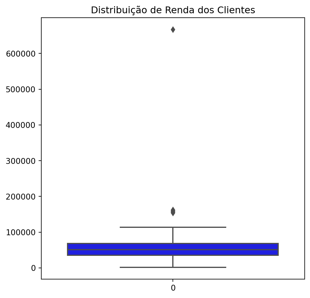
The analysis revealed a significant difference between mean (52,247) and median (51,381). Most notably, the maximum value (666,666) was extremely distant from the third quartile (68,522), a strong indication of outliers. Such extreme values disproportionately affect the mean, making it unreliable for central tendency.
Decision: We chose to replace missing values with the median income, as the median is more robust and less sensitive to outliers, ensuring imputation did not distort the real distribution of income.
Although we imputed missing values using the median, the presence of extreme outliers could still negatively influence models and visualizations. We analyzed the distribution of income further.
Income variable distribution:
Show Code
plt.figure(figsize = (6, 6))plt.title("Customer Income Distribution")sns.boxplot(data = df['Income'], color ='blue')
The $666,666 outlier stood out, and given the dataset size and its singularity, we removed it to reduce noise and improve representativeness.
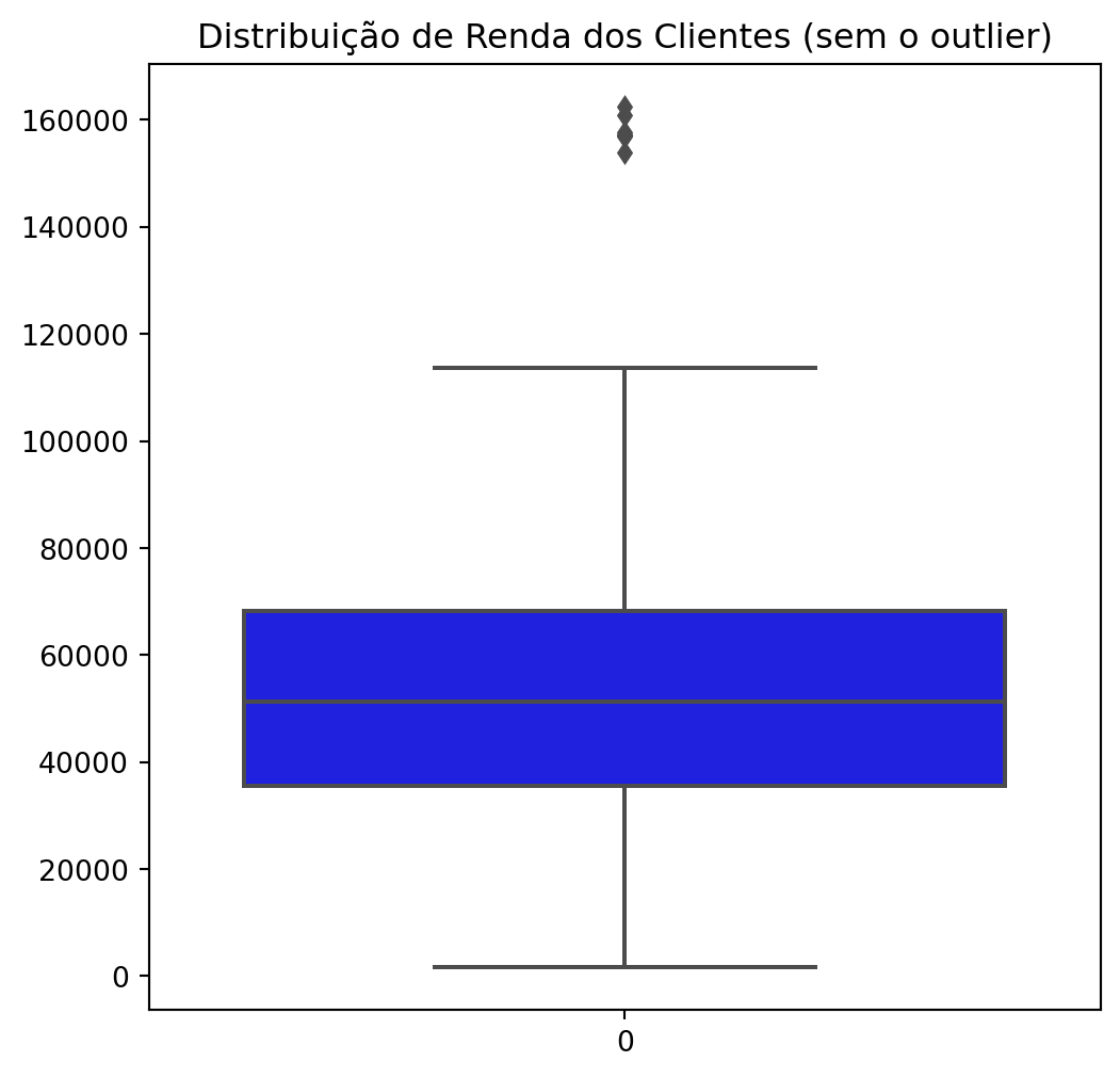
Removing the outlier and plotting again:
Show Code
df = df[df['Income'] !=666666.0]plt.figure(figsize = (6, 6))plt.title("Customer Income Distribution (without outlier)")sns.boxplot(data = df['Income'], color ='blue')
Boxplots before and after confirmed the effectiveness of this intervention, resulting in a cleaner representation of customer income.
Feature Engineering
The creation of new variables, or Feature Engineering, is an important step to enrich the dataset and extract deeper insights. We engineered metrics to capture customer profiles and behaviors.
a) Customer Age at Enrollment (Customer_Age_When_Enrolled)
To understand age distribution at enrollment, we created a column by subtracting birth year (Year_Birth) from enrollment year (Dt_Customer). This metric supports age-targeted campaigns.
While spending was divided across product categories (wine, fruits, meat, fish, sweets, gold), a consolidated “Total_Spent” metric provides a holistic view of customer value.
After aggregation, we dropped Kidhome and Teenhome to avoid redundancy.
Dropping original columns:
Show Code
df = df.drop(['Kidhome', 'Teenhome'], axis =1)
Outlier Re-check with IQR
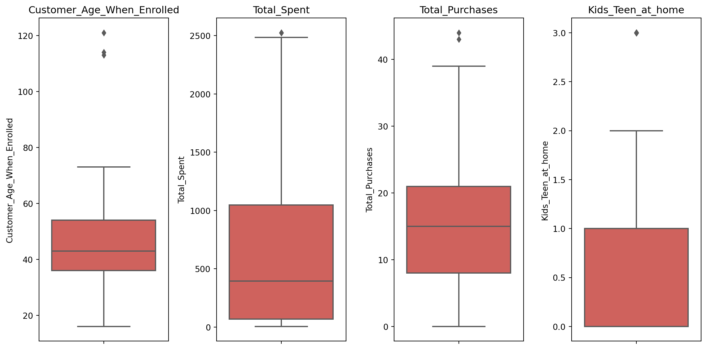
To ensure the quality of the new attributes and existing columns, a new outlier verification was performed using the Interquartile Range (IQR) method for the most relevant features for the analysis (Customer_Age_When_Enrolled, Total_Spent, Total_Purchases, Kids_Teen_at_home). The 2 times IQR rule was applied for a more sensitive detection.
Defining columns of interest, creating the function and applying it to the defined columns for outlier identification:
It was found that only 3 outliers persisted in the Customer_Age_When_Enrolled variable, representing a very low percentage (0.13%) of the dataset.
For better visualization, let’s analyze the boxplot of these variables:
Boxplot of variables of interest:
Show Code
plt.figure(figsize=(12,6))for i, coluna inenumerate(colunas): plt.subplot(1, len(colunas), i+1) sns.boxplot(y=df[coluna]) plt.title(coluna)plt.tight_layout()plt.show()
Identification of found outliers:
Show Code
for coluna in colunas: res = detectar_outliers_iqr(df[coluna]) outliers = res['outliers']ifnot outliers.empty:print(f"\nColuna: '{coluna}'")print(outliers)
These extremely atypical values (ages like 113, 114, and 121 years, likely registration errors) were removed to avoid any noise or distortion in future age analyses, which are crucial for customer segmentation.
The resulting dataset, with 2,236 rows and 30 columns, is now clean, more complete with the new features, and ready for the exploratory analysis phase.
Exploratory Data Analysis and Insight Visualizations
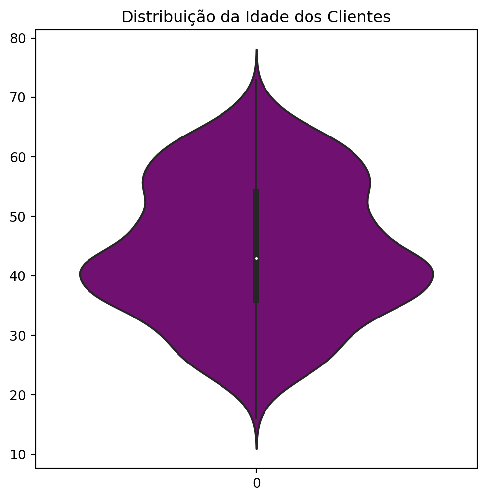
Customer Age Analysis:
Show Code
plt.figure(figsize = (6, 6))plt.title("Customer Age Distribution")sns.violinplot(data = df['Customer_Age_When_Enrolled'], color ='purple')
The distribution of customer ages, visualized through a violin plot, revealed a striking demographic characteristic: the majority of customers are concentrated in the 35 to 45 age group. This data is of utmost importance, as it points to the shopping center’s main market niche, indicating that marketing strategies, product and service selection, and even promotional events should be directed to meet the needs and preferences of this specific demographic group. Customers in this age range generally have greater purchasing power and financial stability, making them a highly valuable target audience.
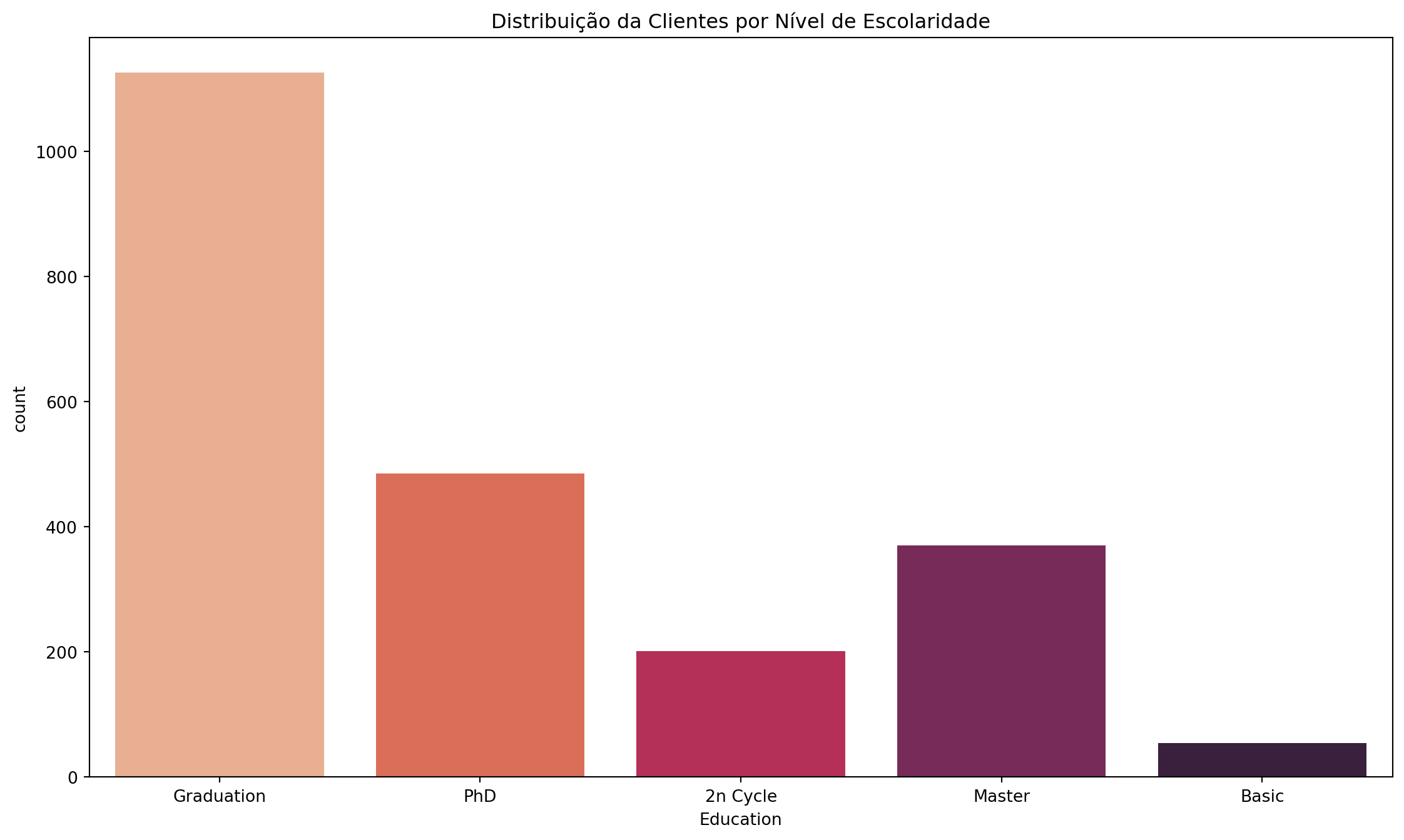
Distribution by Education Level:
Show Code
education_counts = df['Education'].value_counts()plt.figure(figsize = (14, 8))plt.title("Customer Distribution by Education Level")sns.countplot(x = df['Education'], palette ='rocket_r')
The analysis of customer education levels, through a count plot, highlighted the predominance of customers with Bachelor’s degrees, followed by those with PhDs and Master’s degrees. A minority holds only a basic education level. This educational pattern suggests a customer profile that values quality, perhaps with greater access to information and decision-making power regarding their purchases. Understanding this characteristic can influence communication, the type of stores and services offered, and the sales approach, which can be more sophisticated and value-focused.
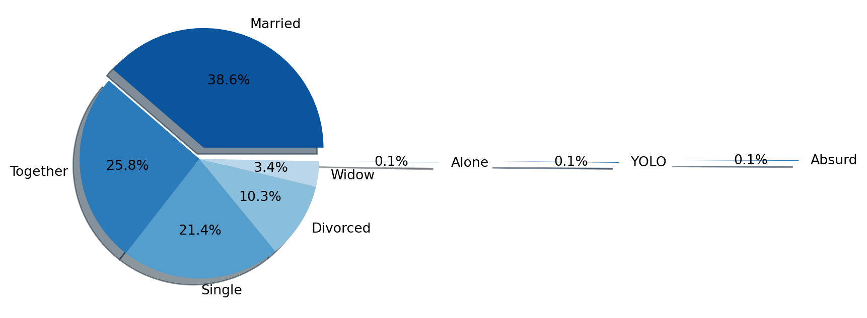
Profile by Marital Status:
Show Code
# Criando um df para armazernar a contagem de cada tipo de estado civilestado_civil = df['Marital_Status'].value_counts().to_frame('Count')# Criando o graficosns.set_palette('Blues_r')plt.figure(figsize = (4, 7))plt.pie(estado_civil['Count'], labels = estado_civil.index, explode = (0.1, 0, 0, 0, 0, 1, 2.5, 4), shadow =True, autopct ='%1.1f%%')plt.show()
The distribution of marital status, illustrated by a pie chart, revealed that most customers are married or living together, followed by single individuals. The predominance of couples suggests that many purchasing decisions may be influenced by family dynamics. This could open opportunities for promotions and events aimed at couples or families, as well as offering products and services that cater to multiple household members.
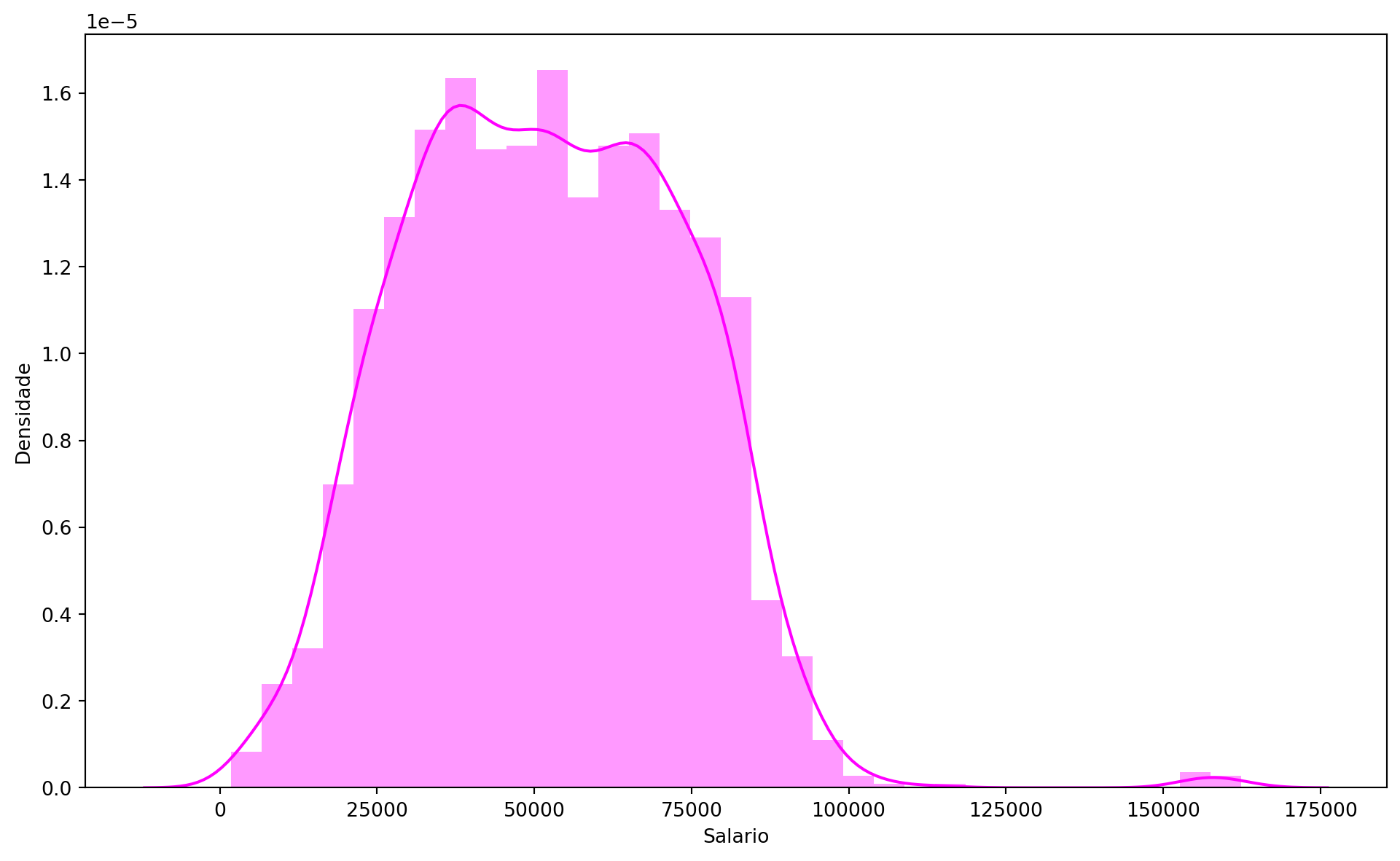
Income Distribution and Spending Patterns:
Show Code
df = df[df['Income'] <200000]plt.figure(figsize = (12,7))sns.distplot(df['Income'], color ='magenta')plt.xlabel('Salary')plt.ylabel('Density')plt.show()
The analysis of income distribution, through a distplot, confirmed that the vast majority of customers have an income around 50,000. Although the distribution is approximately normal,some customers have incomes above 150,000. This concentration indicates a public with medium-to-high purchasing power, who may be sensitive to value propositions but also seek products and services that justify the investment. Higher-income customers, though fewer in number, represent a high-potential segment for premium products and services.
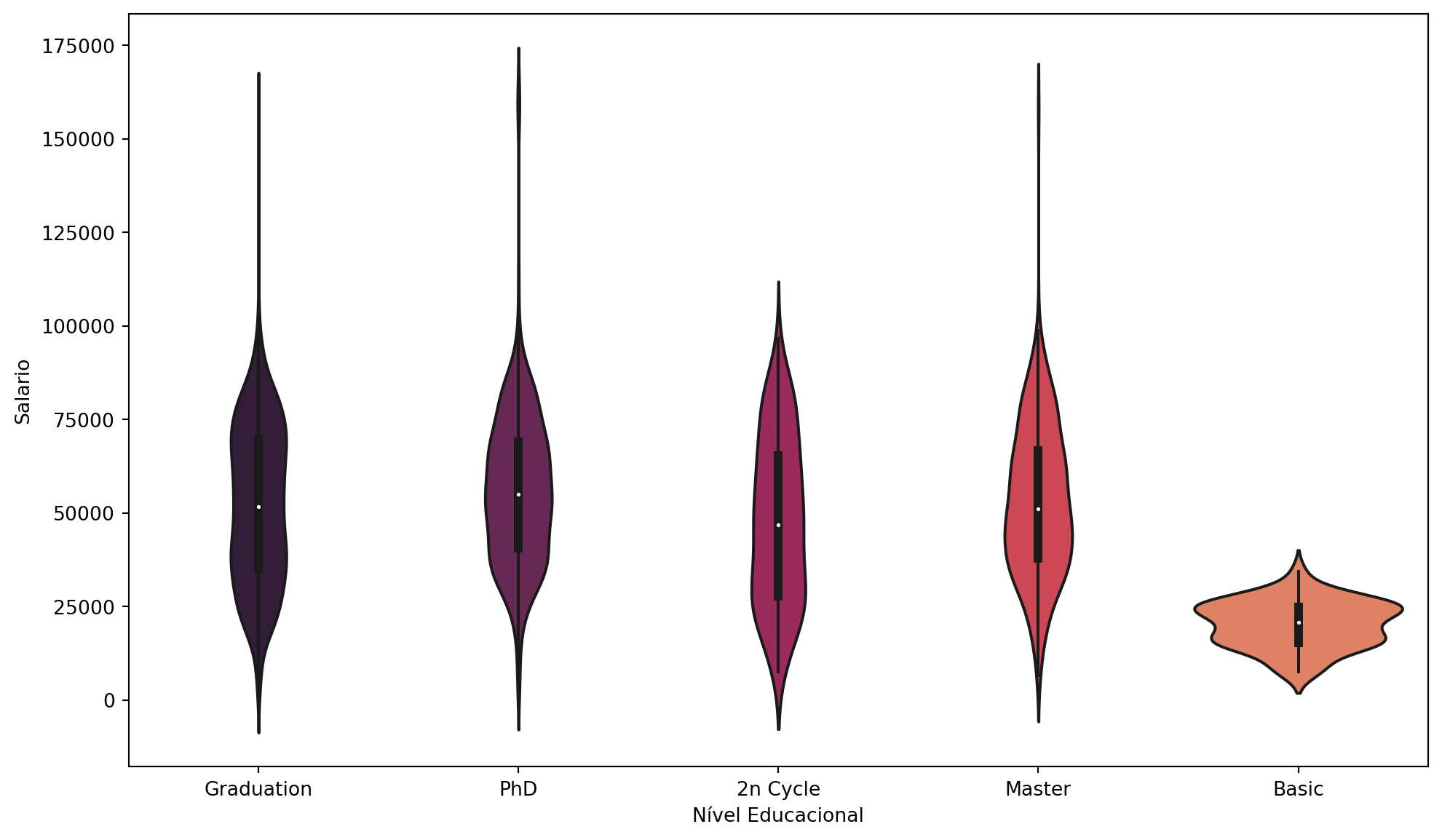
Relationship between Income and Education:
Show Code
sns.set_palette('rocket')plt.figure(figsize = (12, 7))sns.violinplot(y = df['Income'], x = df['Education'])plt.xlabel('Educational Level')plt.ylabel('Salary')plt.show()
The relationship between income and education, explored by a violin plot, validated a common trend: the higher the education level, the higher the income. This correlation reinforces the customer profile as being well-educated with good financial capacity. Stores and brands that align their products and communication with an intellectualized public with aspirations for quality will benefit more in this environment.
Relationship between Income and Spending on Gold Products:
Show Code
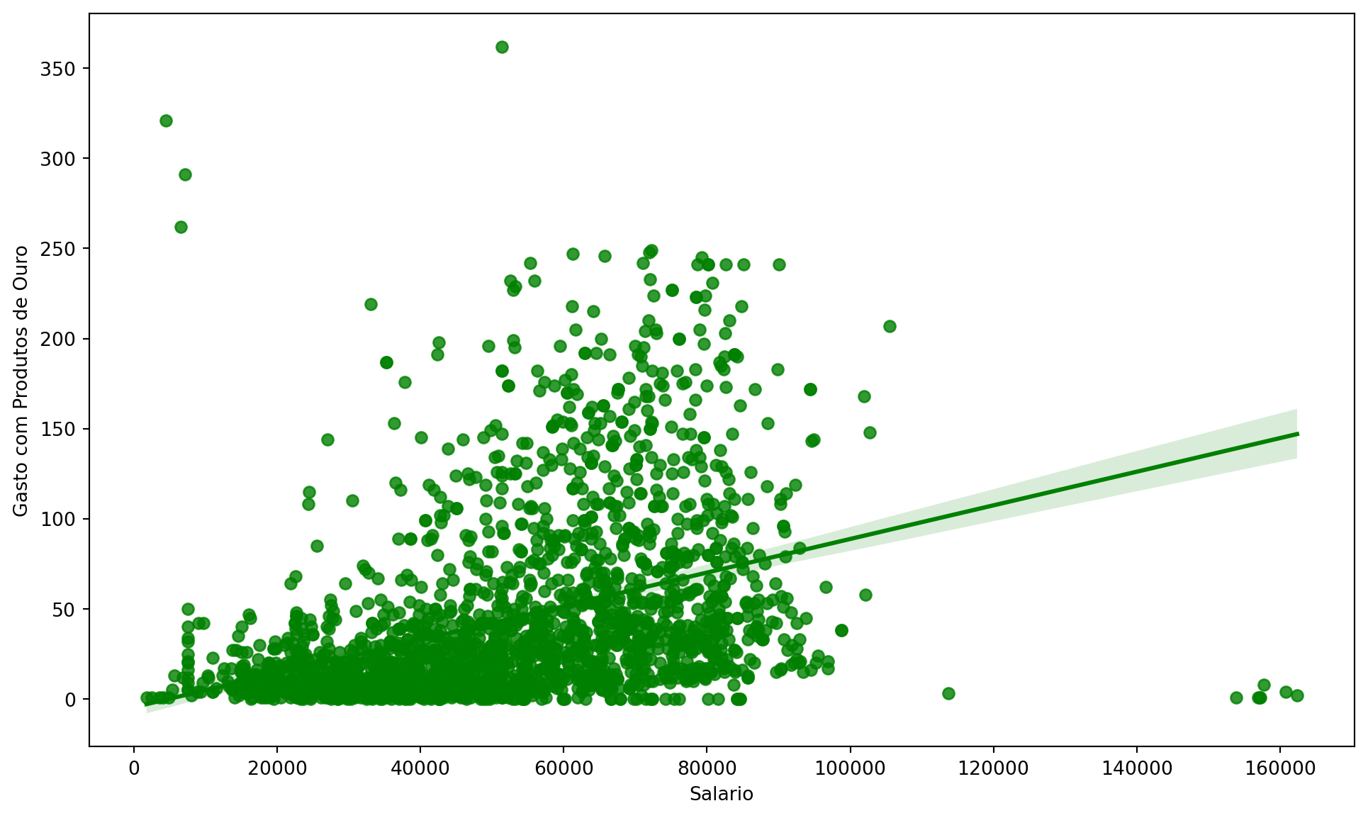
plt.figure(figsize = (12, 7))sns.regplot(x = df['Income'], y = df['MntGoldProds'], color ='green')plt.xlabel('Salary')plt.ylabel('Spending on Gold Products')plt.show()
The relationship between income and spending on gold products, visualized by a regplot, showed a clear positive trend: customers with higher incomes tend to spend more on gold products. This is an interesting indicator of customer purchasing power and taste. Gold and other high-value-added products can be promoted more effectively to the higher-income segment, perhaps through exclusive shopping experiences or differentiated loyalty programs.
Relationship between Income and Total Spending on Purchases:
Show Code
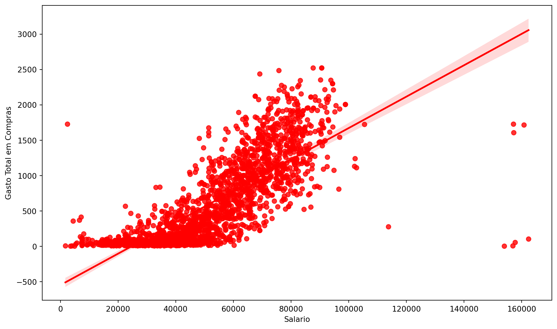
plt.figure(figsize = (12, 7))sns.regplot(x = df['Income'], y = df['Total_Spent'], color ='red')plt.xlabel('Salary')plt.ylabel('Total Spending on Purchases')plt.show()
Even more importantly, the analysis of the relationship between income and total spending on purchases, also through a regplot, confirmed a robust positive relationship: customers with higher incomes naturally contribute a larger volume of spending at the shopping center. This is one of the most fundamental insights, reinforcing the importance of attracting and retaining high-income customers, as they are the backbone of revenue. Strategies aimed at increasing disposable income or the perceived value for these customers can have a direct and significant impact on financial results.
Customer Age at Enrollment Date:
Show Code
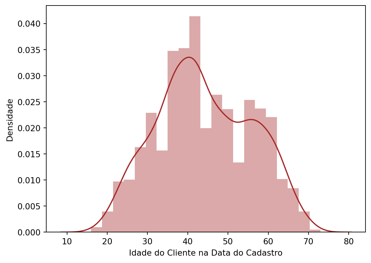
plt.figure(figsize = (7, 5))sns.distplot(df['Customer_Age_When_Enrolled'], color ='brown')plt.xlabel('Customer Age at Enrollment Date')plt.ylabel('Density')plt.show()
The distribution of customer age at the registration date, a distplot, reiterated the concentration of customers in their 40s. This solidifies the idea that the shopping center has a strong appeal to a more mature and established audience, consolidating an important and consistent market niche. Communication and offers should resonate with the interests and lifestyle of this demographic.
Customer Distribution by Country of Origin:
Show Code
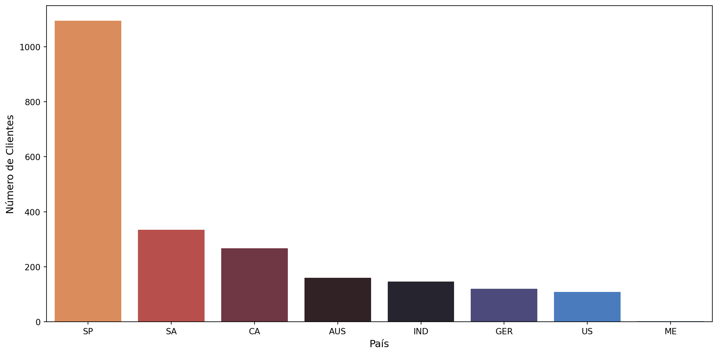
plt.figure(figsize=(12, 6))sns.countplot( x='Country', data=df, palette='icefire_r', order=df['Country'].value_counts().index)plt.xlabel('Country', fontsize=12)plt.ylabel('Number of Customers', fontsize=12)plt.tight_layout()plt.show()
The analysis of customer distribution by country, using a countplot, revealed a clear concentration of customers in the dataset’s country of origin, Singapore, followed by Saudi Arabia and Canada. Singapore’s dominance is expected and reinforces the shopping center’s local base. The significant presence of customers from Saudi Arabia and Canada indicates a potential international or high-income clientele who may be visiting the region. This opens the way for shopping tourism strategies and partnerships with travel agencies, or even adapting offers for specific cultures.
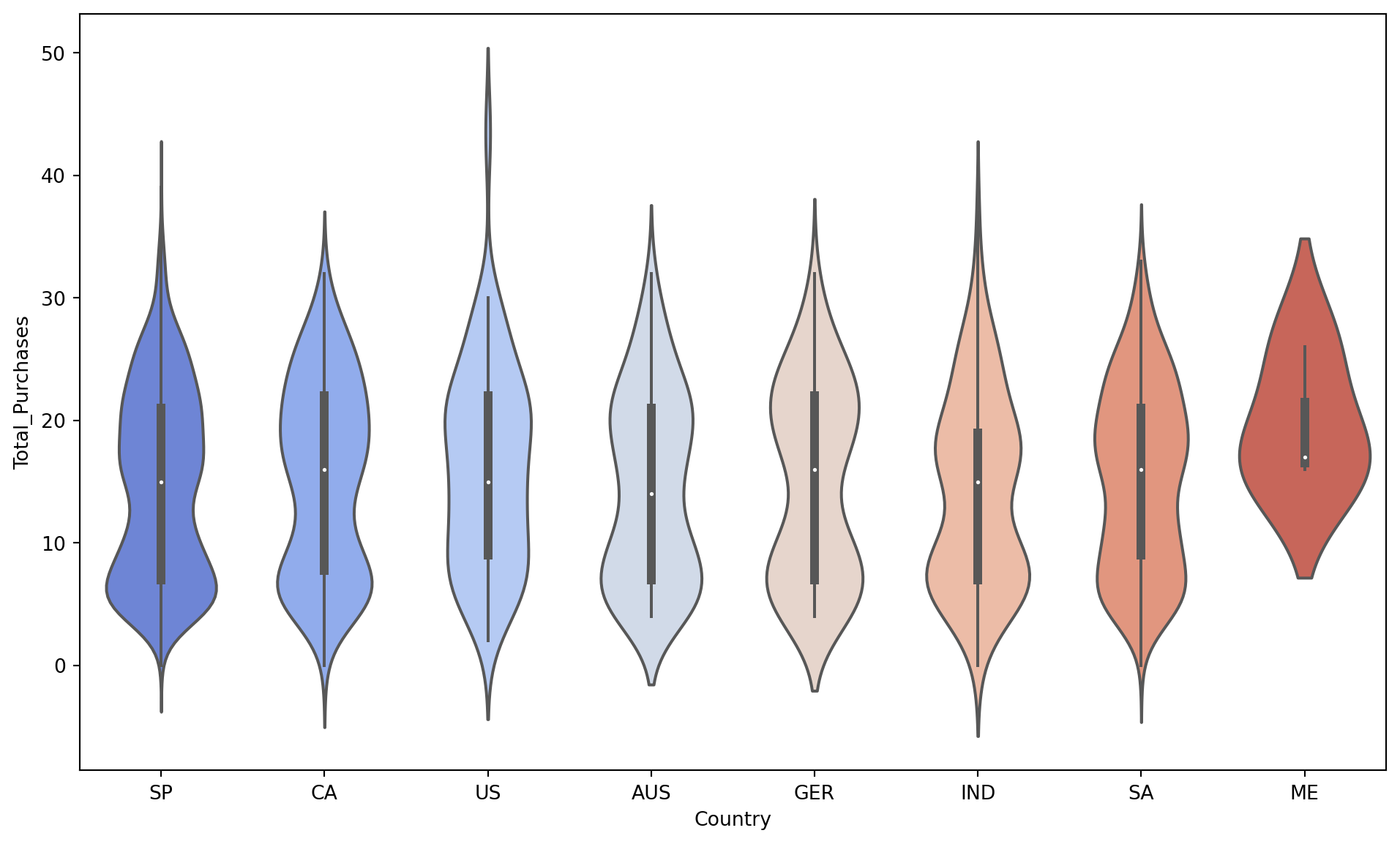
Relationship between Country of Origin and Total Purchases:
A violin plot comparing the country of origin with total purchases showed that, in general, countries exhibit similar purchasing behavior. However, there were notable exceptions: the United States showed some customers with significantly higher purchase values, while Mexico displayed distinctly different behavior from the others. This suggests that, although the average purchasing profile is consistent, there are market niches in specific countries, such as the “super buyers” from the USA, who deserve special attention. For Mexico, a more in-depth study of why its behavior diverges could reveal specific opportunities or challenges.
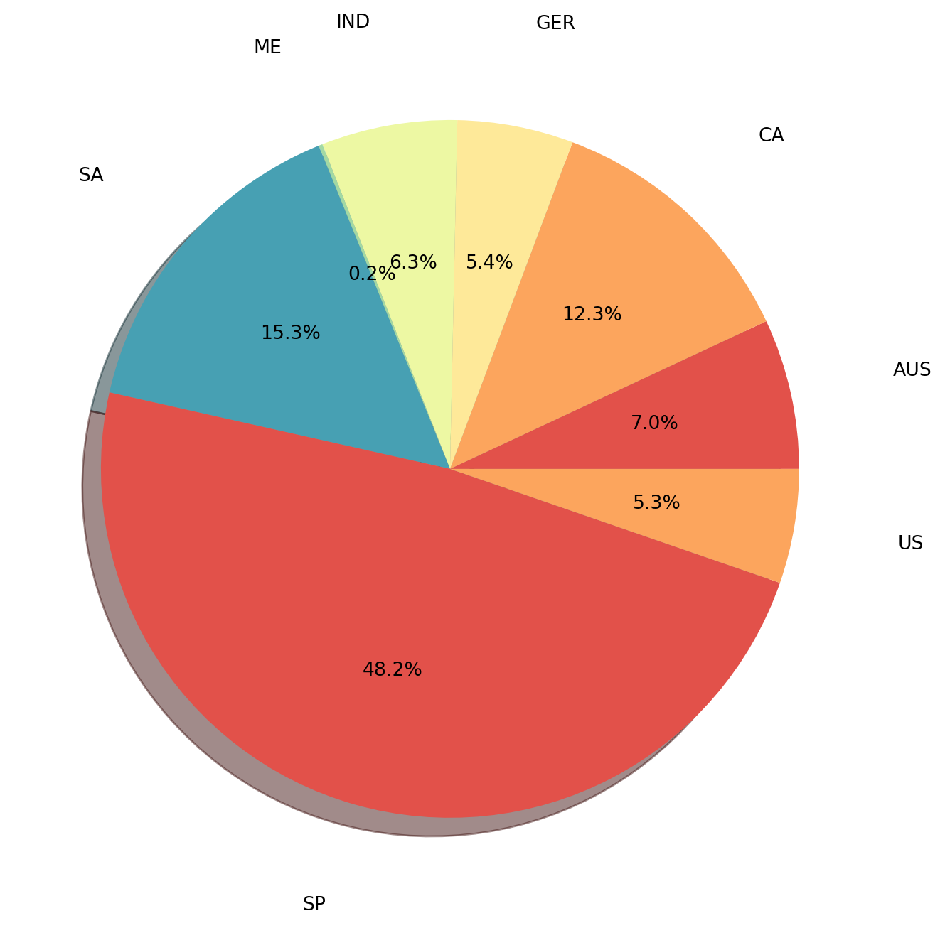
The analysis of total aggregated spending by country, through a pie chart, confirmed what was already intuitive: the majority of revenue comes from Singapore, followed by Saudi Arabia, which together account for almost 55% of total purchases. This concentration of value in two countries reinforces the need to focus retention and engagement efforts on these primary markets. Personalized strategies and loyalty campaigns for customers from Singapore and Saudi Arabia are crucial for the shopping center’s financial health.
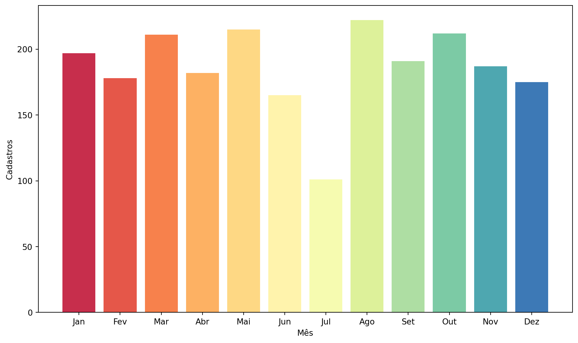
The distribution of customer registrations throughout the months of the year, presented in a bar chart, revealed that the acquisition process is relatively well distributed. There was a slight dip in June and July, which could be seasonal or indicate opportunities for acquisition campaigns during these periods. The stability in monthly registrations is a good sign. The slight declines in June and July could be targets for specific marketing actions to boost acquisition during these months, perhaps with exclusive promotions for new registrations or themed events.
Conclusion
This analysis of the shopping center’s customer profile revealed crucial insights that can guide future business strategies. By understanding who the customers are, where they come from, their purchasing power, and their spending habits, the shopping center can significantly optimize its operations.
Key Project Insights:
Defined Target Audience: The shopping center predominantly attracts an adult audience, aged between 35 and 45, with high education (Bachelor’s, PhD, Master’s) and mostly married or in a stable union. This is its core business and should be the main focus.
Consistent Purchasing Power: The majority of customers have income concentrated around $50,000, with a clear positive correlation between income, education, and total spending (including high-value products like gold). This validates the strategy of focusing on an audience that seeks quality and has investment capacity.
Geographic Customer Base: Although diversified, the customer base is predominantly local (Singapore) with a notable contribution from Saudi Arabia and Canada. This suggests opportunities to optimize strategies for both the domestic market and shopping tourism.
Country-Specific Behaviors: The identification of high-spending customers in the USA and a different pattern in Mexico points to the need for country-segmented approaches to maximize returns.
Acquisition Stability: Customer registrations are well distributed throughout the year, with small dips in June and July, which can be opportunities for targeted acquisition campaigns.
Ultimately, this project highlights how Data Science bridges the gap between raw data and business strategy, empowering retail organizations to remain competitive and customer-centric.”